Chapter 3 Biased transmission: direct bias
In the previous chapters, we have looked at unbiased transmission (Chapter 1) and unbiased and biased mutation (Chapter 2). Let’s complete the set by looking at biased transmission. This occurs when one trait is more likely to be copied than another trait. When the choice depends on the features of the trait, it is often called ‘direct’ or ‘content’ bias. When the choice depends on features of the demonstrators (the individuals from whom one is copying), it is often called ‘indirect’ or ‘context’ bias. Both are sometimes also called ‘cultural selection’ because one trait is selected to be copied over another trait. In this chapter, we will look at trait-based (direct, content) bias.1
3.1 A simple model of directly biased transmission
To simulate biased transmission, following the simulations in Chapter 1, we assume there are two traits \(A\) and \(B\), and that each individual chooses another individual from the previous generation at random. This time, however, we give the traits two different probabilities of being copied: we can call them \(s_a\) and \(s_b\) respectively. When an individual encounters another individual with trait \(A\), they will copy them with probability \(s_a\). When they encounter an individual with trait \(B\), they will copy them with probability \(s_b\).
With \(s_a=s_b\), copying is unbiased, and individuals switch to the encountered alternative with the same probability. This reproduces the results of the simulations when the transmission is unbiased. If \(s_a=s_b=1\), the model is exactly the same as in Chapter 1. The relevant situation in this chapter is when \(s_a \neq s_b\) so that we have biased transmission. Perhaps \(A\) (or \(B\)) is a more effective tool, a more memorable story, or a more easily pronounced word.
Let’s first write the function, and then explore what happens in this case. Below is a function biased_transmission_direct() that implements all of these ideas.
library(tidyverse)

biased_transmission_direct <- function (N, s_a, s_b, p_0, t_max, r_max) {

  output <- tibble(generation = rep(1:t_max, r_max),
                   p = as.numeric(rep(NA, t_max * r_max)),
                   run = as.factor(rep(1:r_max, each = t_max)))

  for (r in 1:r_max) {
    # Create first generation
    population <- tibble(trait = sample(c("A", "B"), N,
                                        replace = TRUE, prob = c(p_0, 1 - p_0)))

    # Add first generation's p for run r
    output[output$generation == 1 & output$run == r, ]$p <-
      sum(population$trait == "A") / N

    for (t in 2:t_max) {
      # Copy individuals to previous_population tibble
      previous_population <- population

      # For each individual, pick a random individual from the previous generation
      demonstrator_trait <-
        tibble(trait = sample(previous_population$trait, N, replace = TRUE))

      # Biased probabilities to copy:
      copy_a <- sample(c(TRUE, FALSE), N, prob = c(s_a, 1 - s_a), replace = TRUE)
      copy_b <- sample(c(TRUE, FALSE), N, prob = c(s_b, 1 - s_b), replace = TRUE)

      # If the demonstrator has trait A and the individual wants to copy A, then copy A
      if (nrow(population[copy_a & demonstrator_trait$trait == "A", ]) > 0) {
        population[copy_a & demonstrator_trait$trait == "A", ]$trait <- "A"
      }

      # If the demonstrator has trait B and the individual wants to copy B, then copy B
      if (nrow(population[copy_b & demonstrator_trait$trait == "B", ]) > 0) {
        population[copy_b & demonstrator_trait$trait == "B", ]$trait <- "B"
      }
      # Get p and put it into output slot for this generation t and run r
      output[output$generation == t & output$run == r, ]$p <-
        sum(population$trait == "A") / N
    }
  }
  # Export data from function
  output
}
Most of biased_transmission_direct() is recycled from the previous models. As before, we initialise the data structure output from multiple runs, and in generation \(t=1\), we create a population tibble to hold the trait of each individual.
The major change is that we now include biased transmission. We first select at random the demonstrators from the previous generation (using the same code we used in unbiased_transmission()) and we store their trait in demonstrator_trait. Then we get the probabilities for copying \(A\) and for copying \(B\) for the entire population, using the same code used in biased_mutation(). Again we have individuals copy the trait at hand with the desired probability.
Let’s run our function biased_transmission_direct(). As before, we can plot the results with the plot_multiple_runs() function that we wrote in the first chapter.
As noted above, the interesting case is when one trait is favoured over the other. We can assume, for example, \(s_a=0.1\) and \(s_b=0\). This means that when individuals encounter another individual with trait \(A\) they copy them 1 out every 10 times, but when individuals encounter another individual with trait \(B\), they never switch. We can also assume that the favoured trait, \(A\), is initially rare in the population (\(p_0=0.01\)) to see how selection favours this initially-rare trait (Note that \(p_0\) needs to be \(>0\); since there is no mutation in this model, we need to include at least some \(A\)s at the beginning of the simulation, otherwise it would never appear).
data_model <- biased_transmission_direct(N = 10000, s_a = 0.1, s_b = 0 ,
                                         p_0 = 0.01, t_max = 150, r_max = 5)
plot_multiple_runs(data_model)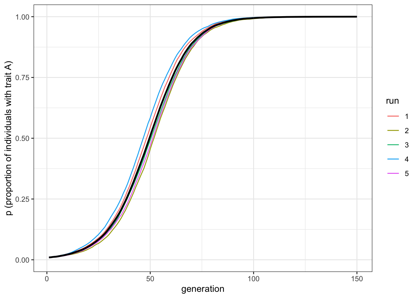
Figure 3.1: Biased transmission generates an s-shaped diffusion curve
With a moderate selection strength, we can see that \(A\) gradually replaces \(B\) and goes to fixation. It does this in a characteristic manner: the increase is slow at first, then picks up speed, then plateaus.
Note the difference from biased mutation. Where biased mutation was r-shaped, with a steep initial increase, biased transmission is s-shaped, with an initial slow uptake. This is because the strength of biased transmission (like selection in general) is proportional to the variation in the population. When \(A\) is rare initially, there is only a small chance of picking another individual with \(A\). As \(A\) spreads, the chances of picking an \(A\) individual increases. As \(A\) becomes very common, there are few \(B\) individuals left to switch. In the case of biased mutation, instead, the probability of switching is independent of the variation in the population.
3.2 Strength of selection
What does the strength of selection depend on? First, the strength is independent of the specific values of \(s_a\) and \(s_b\). What counts is their relative difference, which in the above case is \(s_a-s_b = 0.1\). If we run a simulation with, say, \(s_a=0.6\) and \(s_b=0.5\), we see the same pattern, albeit with slightly more noise. That is, the single runs are more different from one another compared to the previous simulation. This is because switches from \(A\) to \(B\) are now also possible.
data_model <- biased_transmission_direct(N = 10000, s_a = 0.6, s_b = 0.5 ,
                                         p_0 = 0.01, t_max = 150, r_max = 5)
plot_multiple_runs(data_model)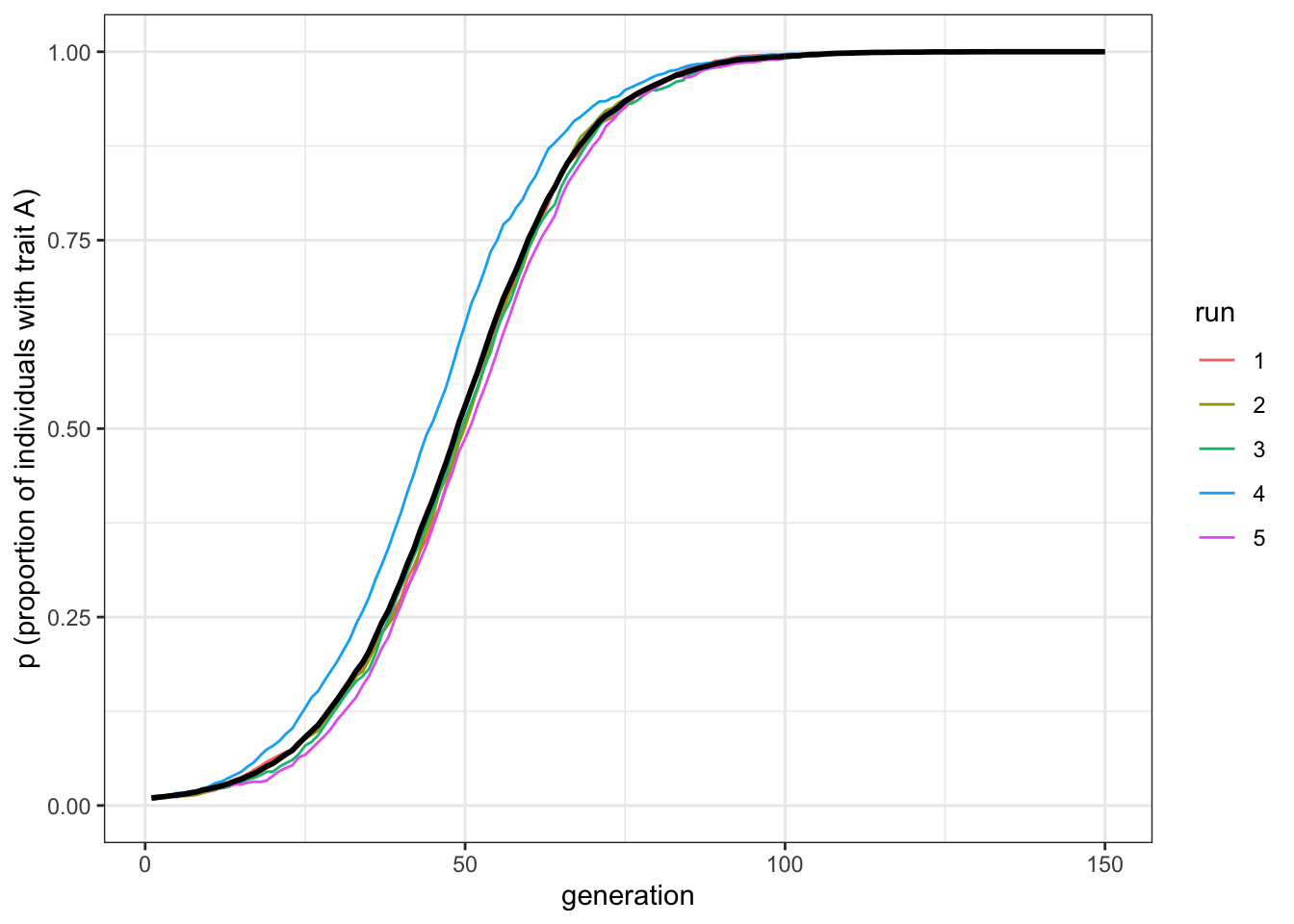
Figure 3.2: Biased transmission depends on the relative difference between the transmission parameters of each trait
To change the selection strength, we need to modify the difference between \(s_a\) and \(s_b\). We can double the strength by setting \(s_a = 0.2\), and keeping \(s_b=0\).
data_model <- biased_transmission_direct(N = 10000, s_a = 0.2, s_b = 0 ,
                                         p_0 = 0.01, t_max = 150, r_max = 5)
plot_multiple_runs(data_model)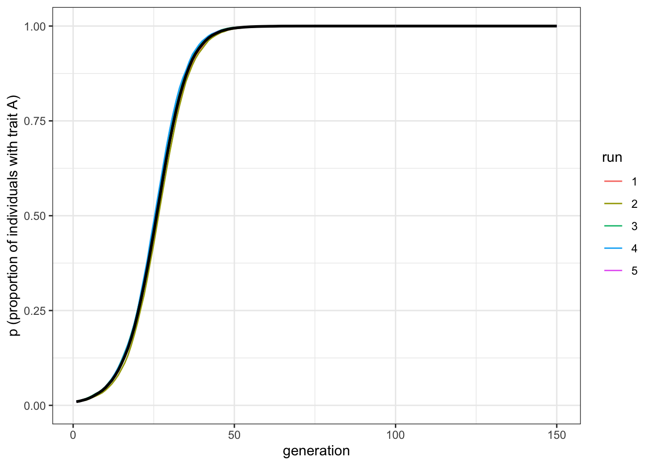
Figure 3.3: Increasing the relative difference between transmission parameters increases the rate at which the favoured trait spreads
As we might expect, increasing the strength of selection increases the speed with which \(A\) goes to fixation. Note, though, that it retains the s-shape.
3.3 Summary of the model
We have seen how biased transmission causes a trait favoured by cultural selection to spread and go to fixation in a population, even when it is initially very rare. Biased transmission differs in its dynamics from biased mutation. Its action is proportional to the variation in the population at the time at which it acts. It is strongest when there is lots of variation (in our model, when there are equal numbers of \(A\) and \(B\) at \(p=0.5\)), and weakest when there is little variation (when \(p\) is close to 0 or 1).
3.4 Further reading
Boyd and Richerson (1985) modelled direct bias, while Henrich (2001) added directly biased transmission to his guided variation / biased mutation model, showing that this generates s-shaped curves similar to those generated here. Note though that subsequent work has shown that s-shaped curves can be generated via other processes (e.g. Reader (2004)), and should not be considered definite evidence for biased transmission.
As an aside, there is a confusing array of terminology in the field of cultural evolution, as illustrated by the preceding paragraph. That’s why models are so useful. Words and verbal descriptions can be ambiguous. Often the writer doesn’t realise that there are hidden assumptions or unrecognised ambiguities in their descriptions. They may not realise that what they mean by ‘cultural selection’ is entirely different from how someone else uses it. Models are great because they force us to specify exactly what we mean by a particular term or process. We can use the words in the paragraph above to describe biased transmission, but it’s only really clear when we model it, making all our assumptions explicit.↩︎