Chapter 13 Demography

In the previous chapters, we have looked at the transmission of information between individuals. We have seen that relatively simple mechanisms at the individual level can affect population-level outcomes (e.g. the fixation of a rare cultural trait). We have also seen the importance of the characteristics of individuals (e.g. for success and prestige bias) in cultural processes. What we have not yet looked at is how the characteristics of the population may affect the outcome of cultural dynamics. In the following three chapters we will have a closer look at how population size (demography, this chapter), population structure (social networks, Chapter 14), and group structured populations with migration (Chapter 15) can influence cultural evolution.

Why does population size matter for cultural evolution? As we have seen in earlier chapters, small populations are prone to random loss of cultural traits due to cultural drift. However, there are other aspects too. For example, innovation might be hard and require many brains to ponder over. Or learning can be error-prone and individuals might often fail to acquire a functional copy of a cultural trait. In this chapter, we will look at how those errors affect information accumulation and how population size is moderating this process.

Several studies have looked at population effects. A well-known study is by Joseph Henrich (2004). His model takes inspiration from the archaeological record of Tasmania, which shows a deterioration of some cultural traits and the persistence of others after Tasmania was cut-off from Australia at the end of the last ice age. Henrich develops a compelling analytical model to show that the same adaptive processes in cultural evolution can result in the improvement and retention of simple skills, but also the deterioration and even loss of complex skills. In the following section, we will take a closer look at his model.

13.1 The Tasmania Case

The main idea of Henrich’s model is the following: information transmission from one generation to another (or from one individual to another, here it does not make a difference) has a random component (error rate) that will lead to most individuals failing to achieve the same skill level, \(z\), as their demonstrators, whereas a few will match and—even fewer—exceed that skill level. Imagine a group of students who try to acquire the skills to manufacture an arrowhead. As imitation is imperfect, and memorizing and recalling action sequences is error-prone, some students will end up with inferior arrowheads when compared to their demonstrator (we assume students will always learn from the best), and only a few will match or improve upon the demonstrator’s skill.

To simulate imperfect imitation, Henrich’s model uses random values from a Gumbel distribution. This distribution is commonly used to model the distribution of extreme values. Its shape is controlled by two parameters: \(\mu\) (location) and \(\sigma\) (scale, sometimes also denoted as \(\beta\)). Varying \(\mu\) affects how tricky it is to acquire a given skill. If we subtract an amount \(\alpha\) from \(\mu\) we move the distribution to the left, and so fewer individuals will acquire a skill level that is larger than that of the cultural model. The larger \(\alpha\) the less likely it is to acquire a given skill level. Varying \(\sigma\) on the other hand affects the width of the distribution, and so whether imitators make very similar or systematic mistakes (small \(\sigma\), narrow distribution) or whether errors are very different from each other (large \(\sigma\), wide distribution). By using different values for \(\alpha\) and \(\sigma\), we can simulate different skill complexity and imperfect imitation. Intuitively, whether the average skill level of a population increases, persists, or decreases depends on how likely it is that some imitators will achieve a skill that exceeds the current cultural model. An illustration of Gumbel distributions for a complex and a simple skill is provided in the figure below.

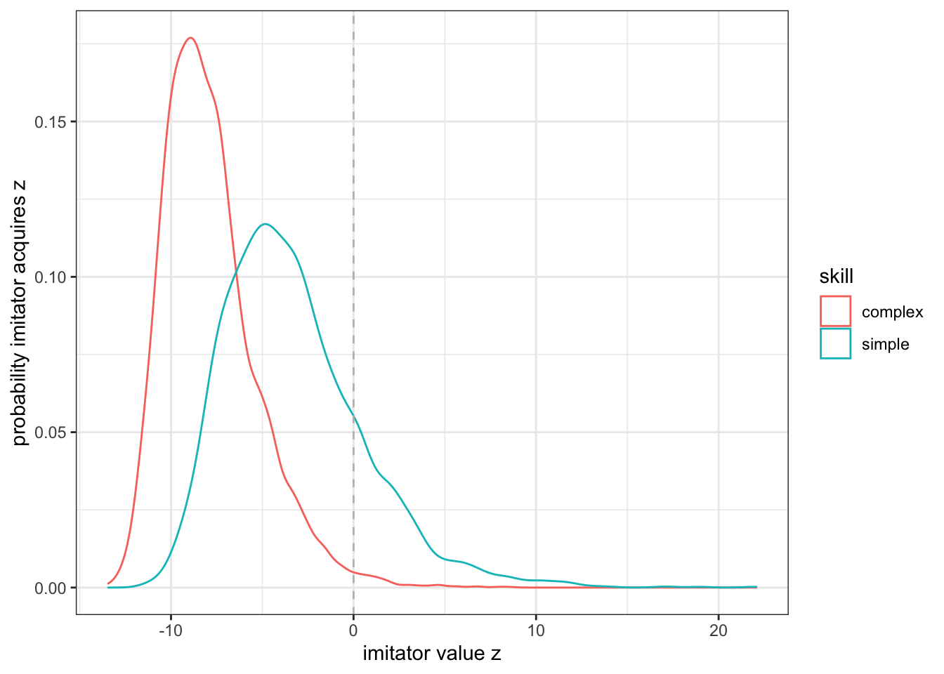
Figure 13.1: Shown are the probability distributions to acquire a specific skill level (\(z\), x-axis) for two different skills (a simple one that is easy to learn, and a complex one that is harder to learn). Given that learning is error-prone more individuals will acquire a skill level that is lower than that of a cultural model (its level is indicated by the vertical dashed line) through imitation (left of the dashed line). A few individuals will achieve higher skill levels (right of the dashed line). For the complex skill, the probability to be above the skill level of the cultural model is lower (smaller area under the curve) than for simple skills.

In addition to skill complexity, whether a population can maintain a certain skill level also depends on how many individuals try to learn the skill (i.e. how many values are drawn from the distribution). The smaller the pool of learners, the fewer individuals will achieve a higher skill level and so, over time the skill level will decrease. Henrich provides an analytical model to explain how societies below a critical size (of cultural learners) might lose complex (or even simple) cultural skills over time. Here, we will re-create these results using an individual-based model.

13.2 Modelling the Tasmania Case

We begin with a population with \(N\) individuals. Each individual has a skill level \(z\). In each round, we determine the highest skill level in the population, \(z_{\text{max}}\). We will then draw new values of \(z\) for each individual in the population. We draw these values from Gumbel distribution where the new mean is the same as the skill level of the most skilled individual minus \(\alpha\), i.e. \(\mu = z_{\text{max}} - \alpha\). To keep track of the simulation we will store the average proficiency \(\bar z\) and the change in average proficiency \(\Delta \bar z\).

You will notice that we load a new library, called extraDistr. Thie package provides a function to draw random values from a Gumble function (rgumbel()), similar to functions we used before (e.g. runif()). We will have to define the shape of the distribution by providing the two values \(\mu\) (location) and \(\sigma\) (scale).

Next, we set the some of the parameters that we need to run the simulation, that is, population size N and the number of simulation turns t_max. We also create some data structures to store the skill level z for each individual, and the reporting variables z_bar and z_delta_bar for average skill level and the change of the average skill level, respectively.

We also set the parameters for the Gumbel distribution, here \(\sigma=1\) and \(\alpha=7\).

Finally, we write down a very basic learning loop. The first step in this for() loop is to draw new values of z and store them in z_new. We then calculate the mean of the new skill levels and the change compared to the previous time step and finally update all values stored in z.

library(tidyverse)
library(extraDistr)

# Set population size
N <- 1000
# Set number of simulation rounds
t_max <- 5000
# Draw random values from a uniform distribution to initialise z
z <- rep(1, N)
# Set up variable to store average z
z_bar <- rep(NA, t_max)
# Set up variable to store change in average z
z_delta_bar <- rep(NA, t_max)

# Set parameters for Gumbel distribution
sigma <- 1
alpha <- 7

for(r in 1:t_max){
  # Calculate new z
  z_new <- rgumbel(n = N, mu = max(z) - alpha, sigma = sigma)
  # Record average skill level
  z_bar[r] <- mean(z_new)
  # Record average change in z
  z_delta_bar[r] <- mean(z_new - z)
  # Update z
  z <- z_new
}

Let us now plot the result of this simulation run. We first transform the output data structures in a tibble, so that it can be conveniently plotted with ggplot:

z_delta_bar_val <- tibble(x = 1:length(z_delta_bar), y = z_delta_bar)
ggplot(z_delta_bar_val) + 
  geom_line(aes(x = x, y = y)) +
  xlab("time") +
  ylab("change in z") +
  geom_hline(yintercept = mean(z_delta_bar_val$y), col = "grey", linetype = 2) +
  theme_bw()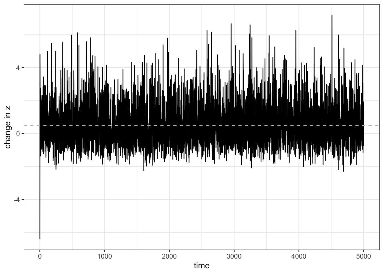

Figure 13.2: While \(\bar z\) is sometimes above and sometimes below \(0\), it is on average postive (dashed line), which indicated that the average skill level of the population increases.

We find that \(\Delta \bar z\) quickly plateaus at about 0.5 (grey dashed line). As this is \(>0\), on average the population will improve its skill over time. We can see that this is the case when we plot the average skill level over time:

z_bar_val <- tibble(x = 1:length(z_bar), y = z_bar)
ggplot(z_bar_val) + 
  geom_line(aes(x = x, y = y)) +
  xlab("time") +
  ylab("average skill-level") +
  theme_bw()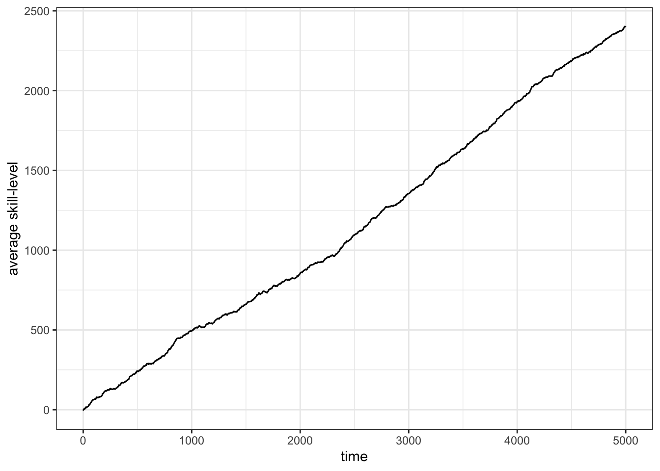

Figure 13.3: For the given parameter (\(\alpha=7\), \(\sigma=1\)) the average skill-level increases continously.

As in the previous chapters, we can now write a wrapper function that allows us to execute this model repeatedly and for different parameters. In the following, we will use a new function: lapply(). There is a series of so-called apply functions in the R programming language that ‘apply’ a function to the elements of a given data object. Generally, these functions take an argument X (a vector, matrix, list, etc.) and then apply the function FUN to each element. Here, we use lapply on a vector 1:R_MAX, that is, a vector of the length of the number of repetitions that we want. What will happen is that lapply() will execute the function that we will provide exactly R_MAX times, and then return the result of each calculation in a list at the end. We could also use a for() loop just as we have done in the previous chapters. However, the advantage of using the apply function over the loop is that simulations can run independently from each other. That is because the second simulation does not have to wait for the first to be finished. In contrast, we could not use the apply function for the individual turns. Here the second simulation step does rely on the results of the first step. In this case, all simulation steps have to be calculated in sequence.

Have a look at our demography_model() wrapper function:

demography_model <- function(T_MAX, N, ALPHA, SIGMA, R_MAX){
  res <- lapply(1:R_MAX, function(repetition){
                  z <- rep(1, N)
                  z_delta_bar <- rep(NA, T_MAX)
                  for(turn in 1:T_MAX){
                    z_new <- rgumbel(n = N, mu = max(z) - ALPHA, sigma = SIGMA)
                    z_delta_bar[turn] <- mean(z_new - z)
                    z <- z_new
                  }
                  return(mean(z_delta_bar))
                })
  mean(unlist(res))
}

Our function demography_model() requires a set of arguments to run (note, it can be useful to capitalize arguments of a function to differentiate between those values that are calculated within a function (not capitalized) and those that have been provided with the function call). The lapply() function will run independent simulations which we have discussed above (i.e. setting up a population of individuals with skill level z, updating these values, and calculating the change in average skill level). The last step is to calculate the mean of z_delta_bar, i.e. the average of the change of the mean skill level. This value is calculated for each repetition. lapply() returns all of these values in a list called res. As we are interested in the average change of the skill level across all repetitions, we first turn this list into a vector (using the unlist() function) and then average all values.

Let us now use the demography_model() function to run repeated simulations for different population sizes and different skill complexity. Here, we use the following parameters for the skill complexities: \(\alpha=7, \sigma=1\) (simple) and \(\alpha=9, \sigma=1\) (complex).

We first define a variable, sizes, for the different population sizes. We are then again relying on the magic of the lapply() function. As above, the reason is that we can let simulations with different population sizes run independently from each other. Note that we provide sizes as our X argument, and demography_model() as the FUN function argument. Our demography_model() itself requires further arguments to run. In the lapply() function we can simply add them at the end. They will be directly passed on to demography_model() when we execute the lapply() function.

In the last line of this chunk, we create a tibble that will hold the final results of the simulations for each skill and the different population sizes.

sizes <- c(2, seq(from = 100, to = 6100, by = 500))

simple_skill <- lapply(X = sizes, FUN = demography_model, 
                       T_MAX = 200, ALPHA = 7, SIGMA = 1, R_MAX = 20)

complex_skill <- lapply(X=sizes, FUN=demography_model, 
                        T_MAX = 200, ALPHA = 9, SIGMA = 1, R_MAX = 20)

data <- tibble(N = rep(sizes, 2), 
               z_delta_bar = c(unlist(simple_skill), 
                               unlist(complex_skill)), 
               skill = rep(c("simple","complex"), each = length(sizes)))

Let us now plot the results:

ggplot(data) + 
  geom_line(aes(x = N, y = z_delta_bar, color = skill)) +
  xlab("effective population size") + 
  ylab("change in average skill level, delta z bar") + 
  geom_hline(yintercept = 0) + 
  theme_bw()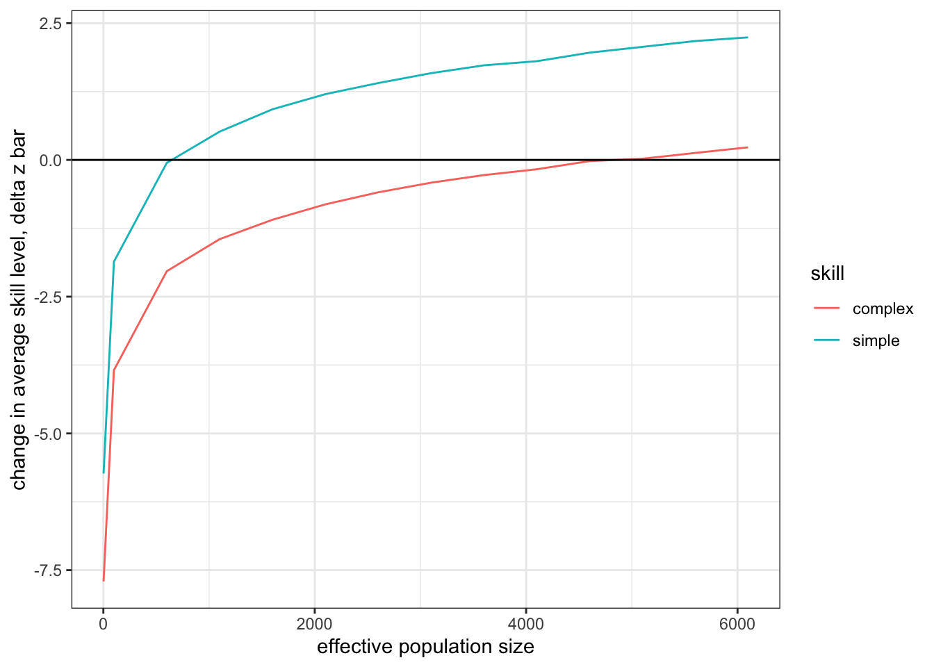

Figure 13.4: For a simple skill, effective populaton size (at which the skill can be just maintained in a population) is much smaller than the population that is required to maintain a complext skill.

In the figure above we can see that, for simple skills, the change in average skill level becomes positive (where it intercepts the x-axis) at much smaller population sizes than the complex skill. This implies that simple skills can be maintained by much smaller populations, whereas larger populations of learners are required for complex skills.

13.3 Calculating critical population sizes based on skill complexity

Henrich calls the minimum population size required to maintain a skill the critical population size, \(N^\star\). How can we calculate \(N^\star\) for different skill complexities? We could run simulations for many more population sizes and find the one where \(\Delta \bar z\) is closest to zero. Alternatively, let us first plot the previous results but with a logarithmix x-axis. The resulting graphs are almost linear.

ggplot(data) + 
  geom_line(aes(x = log(N), y = z_delta_bar, color=skill)) +
  xlab("log(effective population size)") +
  ylab("change in average skill level, delta z bar") + 
  geom_hline(yintercept = 0) + 
  theme_bw()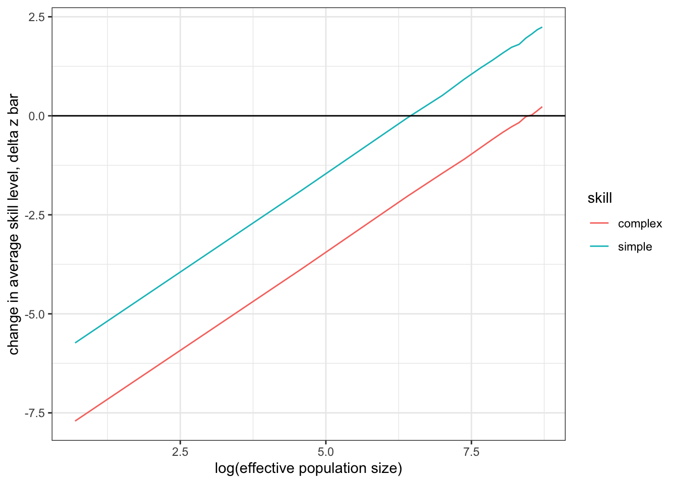

Figure 13.5: The same results as in Figure 13.4 but using log on population sizes.

Thus, we could use a linear fit and then solve for \(y = 0\) to calculate \(N^\star\). To do this we use the lm() function, which fits a linear model to the data that we provide. It takes a formula argument that identifies the ‘response variable’ (here z_delta_bar) and the ‘predictor variable’ (here log(N)). The two variables are separated with a ~ sign. To calculate a fit just for the data points of the simple skill simulation, we only hand over that part of the data where the skill column contains the term simple.

# Create linear regression for the change in average skill level in response to population size
fit <- lm(formula = z_delta_bar ~ log(N), 
          data = data[data$skill == "simple",])
fit

## 
## Call:
## lm(formula = z_delta_bar ~ log(N), data = data[data$skill == 
##     "simple", ])
## 
## Coefficients:
## (Intercept)       log(N)  
##     -6.4284       0.9951

The result provides information about the linear regression. Here, we are interested in the intercept with the y-axis and the inclination of the linear regression, both of which are displayed under Coefficients. We can calculate the point at which our regression line crosses the x-axis using the linear function \(y = mx+b\), setting \(y=0\) and then transforming, such that \(x=-\frac{b}{m}\), where \(b\) is the y-axis intercept, and \(m\) is the inclination.

# Solve for y = 0 by using the coefficients of the linear regression:
b <- fit$coefficients[1]
m <- fit$coefficients[2]
N_star_simple <- exp(-(b / m))

# And the same calculation for the complex skill
fit <- lm(formula = z_delta_bar ~ log(N), 
          data = data[data$skill == "complex",])
N_star_complex <- exp(-(fit$coefficients[1] / fit$coefficients[2]))

Note that we need to take the exponent (exp()) of the resulting value to revert the log function that we applied to the population size. We see that a simple skill with a low alpha to sigma ratio requires a minimum population size of about 639, whereas a much large population size is required to maintain a complex trait (about 4806). (You can visualise those results by writing N_star_simple and N_star_complex.) When you go back to Figure 13.4 you can see that these points correspond with the graphs of the simple and complex skill crossing the x-axis.

Let us now calculate the \(N^\star\) values for different skill complexities and different population sizes. We first set up the parameter space using expand.grid(). This function essentially creates all possible combinations of all the variables we hand over. In our case, we want all possible combinations of the different population sizes N and skill complexities, which we will vary using different values for \(\alpha\). Therefore, executing this function will return a two-column (for N and alpha) data structure, stored in simulations. We can inspect the first lines with the function head():

# Run simulation for the following population sizes
sizes <- seq(from = 100, to = 6100, by = 500)

# Run simulation for the following values of alpha
alphas <- seq(from = 4, to = 9, by = .5)

simulations <- expand.grid(N = sizes, alpha = alphas)
head(simulations)

##      N alpha
## 1  100     4
## 2  600     4
## 3 1100     4
## 4 1600     4
## 5 2100     4
## 6 2600     4

Now we can run simulations for all combinations of population sizes and skill complexities:

z_delta_bar <- lapply(X = 1:nrow(simulations), FUN = function(s){
                  demography_model(T_MAX = 200, 
                                   N = simulations[s, "N"], 
                                   ALPHA = simulations[s, "alpha"], 
                                   SIGMA = 1, 
                                   R_MAX = 5)
  })
# Add results to population size and skill complexity
data <- cbind(simulations, z_delta_bar=unlist(z_delta_bar))

Finally, let us fit a linear regression to each skill complexity to determine the according critical population size \(N^\star\):

n_stars <- lapply(X = unique(data$alpha), FUN = function(alpha){
                      # Only use the results with identical value for alpha
                      subset <- data[data$alpha == alpha,]
                      # Fit regression
                      fit <- lm(formula = z_delta_bar ~ log(N), data = subset)
                      # Solve for n star
                      n_star <- exp(solve(coef(fit)[-1], -coef(fit)[1]))
                      return(n_star)
                    })
# Combine all results in a single tibble
results <- tibble(n_star = unlist(n_stars), alpha = unique(data$alpha))

Now, we plot the critical population size as a function of the skill complexity \(\alpha\) over \(\sigma\). Note, that the x-axis label contains Greek letters. There are at least two ways to get ggplot to display Greek letters. The most simple way is to type the Unicode equivalents of the symbols and letters. In our case this would look like this: xlab("\u03b1 / \u03C3"). Alternatively, we can use the expression() function, which will turn the names of Greek letters into the respective letter from the Greek alphabet:

ggplot(results, aes(x = alpha, y = n_star)) + 
  geom_line() + 
  xlab(expression(alpha/sigma)) +
  ylab("critical populaton size, N*") + 
  theme_bw()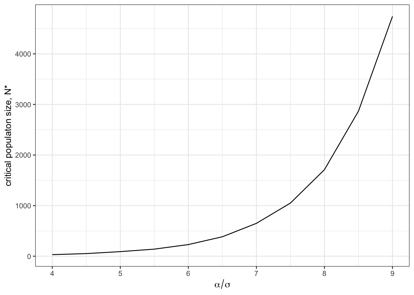

Figure 13.6: The critical population size, \(N^\star\), increases exponentially as skill complexity increases.

It is interesting to observe that the critical population size increases exponentially with skill complexity. This also suggests that all being equal very high skill levels will never be reached by finite population sizes. However, different ways of learning (e.g. teaching) could considerably decrease \(\alpha\) and \(\sigma\) over time and so allow high skill levels.

13.4 Summary of the model

In this chapter, we looked at the interplay between population size and a population’s skill level for a certain trait. Similar to the model in the [Chapter 8][Rogers paradox], the above model is very simple and is making many simplifying assumptions. Nevertheless, it provides an intuitive understanding of how population size changes can affect the cultural repertoire of a population, and how it can be that simple skills thrive, while complex ones disappear. In the next chapter, we will discuss the importance of social networks, i.e. who can interact with whom. We will see that this will also have an effect (additional to the population size). In this chapter, we also introduced several new R functions and programming styles. Most importantly, we used lapply() instead of the usual for loops to run multiple runs of the simulations. We used a different notation for function parameters (all capital letters) to distinguish them from the same values that are calculated within a function).

13.5 Further readings

Henrich (2004) provides a detailed analytical model of the simulation described in this chapter. Powell, Shennan, and Thomas (2009) is an extension to Henrich’s model that incorporates sub-populations with varying densities. Shennan (2001) is another modelling paper that suggests that innovations are far more successful in larger compared to smaller populations. Ghirlanda, Enquist, and Perc (2010) investigates the interplay between cultural innovations and cultural loss. See Shennan (2015) for a general overview of a variety of approaches and questions in studies of population effects in cultural evolution.