Chapter 12 Traits inter-dependence

In real life, the relationship a cultural trait has with other, coexisting, cultural traits, is important to determine its success. Nails will enjoy much cultural success in a world where hammers are present, and less in a world where they are not. Being against abortion in contemporary US is strongly correlated to being religious, which, in turn, is (less strongly) correlated with not supporting same-sex marriage. Of course, not all these relationships are stable in time, and they can also be themselves subject to cultural change. In this chapter, we will explore how simple relationships between traits can be modelled, and how they can influence cultural evolution.

12.1 Compatible and incompatible traits

We can start by assuming that, when an observer meets a demonstrator, the observer evaluates the relationships of the traits of the demonstrator with its own traits, and use this information to decide whether to copy or not. For example, if the observer has the trait ‘being religious’ and the demonstrator the trait ‘being pro abortion,’ copying will be less likely to happen than if the demonstrator has the trait “being against abortion.”

We can imagine a simple scenario when there are only two possible relationships between two traits: they are compatible, meaning that the presence of one trait will reinforce the presence of the other, or incompatible, meaning the opposite. In addition, the relationship is symmetric: if trait A favours trait B, and conversely if trait B favours trait A (the same holds for the case of incompatibility). Finally, we assume that each trait is compatible with itself, simply meaning that, if both the observer and the demonstrator have trait A the probability to copy trait B will increase.

In a simple world with only four traits, we can represent trait relationships with a symmetric matrix, as the one below, where \(+1\) denotes compatibility, and \(-1\) denotes incompatibility.

Traits	A	B	C	D
A	+1	+1	-1	-1
B	+1	+1	-1	-1
C	-1	-1	+1	+1
D	-1	-1	+1	+1

In this case, traits A and B are compatible with each other but incompatible with C and D. The same is true for C and D, which are compatible with each other but incompatible with A and B.

We can construct this matrix in R, by indicating one-by-one the values we want to fill in, and the number of rows and columns the matrix needs to have. As usual, we can check the resulting matrix by writing its name and hitting the return key.

library(tidyverse)
my_world <- matrix(c(1,1,-1,-1,1,1,-1,-1,-1,-1,1,1,-1,-1,1,1), nrow = 4, ncol = 4)
my_world

##      [,1] [,2] [,3] [,4]
## [1,]    1    1   -1   -1
## [2,]    1    1   -1   -1
## [3,]   -1   -1    1    1
## [4,]   -1   -1    1    1

Given this simple way of representing a world of compatibilities among traits, we can write our model.

traits_inter_dependence <- function(N, t_max, k, mu, p_death, world){
  output <- tibble(trait = rep(c("A","B","C","D"), each = t_max), 
                   generation = rep(1:t_max, 4), 
                   p = as.numeric(rep(NA, t_max * 4)))    
  
  population <- matrix(0, ncol = 4, nrow = N)
  
  output[output$generation == 1 ,]$p <- colSums(population) / N
  
  for(t in 2:t_max){
    
    # Innovations
    innovators <- sample(c(TRUE, FALSE), N, prob = c(mu, 1 - mu), replace = TRUE) 
    innovations <- sample(1:4, sum(innovators), replace = TRUE)
    population[cbind(which(innovators == TRUE), innovations)] <- 1
    
    # Copying
    demonstrators <- sample(1:N, replace = TRUE)
    demonstrators_traits <- sample(1:4, N, replace = TRUE)
    
    for(i in 1:N){
      if(population[demonstrators[i], demonstrators_traits[i]]){
        compatibility_score <- sum(world[demonstrators_traits[i], population[i, ] != 0])
        copy <- (1 / (1 + exp(-k*compatibility_score))) > runif(1)
        population[i,demonstrators_traits[i]] <- 1 * copy
      }
    }
    
    # Birth/death
    replace <- sample(c(TRUE, FALSE), N, prob = c(p_death, 1 - p_death), replace = TRUE)
    population[replace, ] <- 0
    
    # Output
    output[output$generation == t ,]$p <- colSums(population) / N
  }
  # Export data from function
  output
}

As in the previous chapter, the simulation starts with no traits, and individuals introduce them with random innovations, the rate of which is regulated by the parameter \(\mu\). Individuals are replaced by culturally-naive newborns with a probability \(p_\text{death}\). There are two major differences from the previous model. One is that the function accepts a parameter, called world, a four-by-four matrix of compatibilities between traits (thus the compatibilities can change, but not the actual number of traits). The second is in the copying procedure.

As in the previous chapter, one trait is randomly selected to be observed from a demonstrator and, if the demonstrator i has it (population[demonstrators[i], demonstrators_traits[i]]), we calculate the ‘compatibility score.’ The compatibility score is the sum of the compatibilities of all the traits of the observer towards the traits of the demonstrator, using the world matrix. If, for example, both observer and demonstrator have A and B (and only A and B), the compatibility would be \(2\), if the observer has A and B and the demonstrator C and D, the compatibility would be \(-2\) and so on. In the next line, the compatibility score is transformed in the actual probability to copy with a logistic function. This is a useful trick to transform possibly unbounded positive and negative values to be between \(0\) and \(1\):

\[P_\text{copy} = \frac{1}{1 + e^{-kC}} \hspace{30 mm}(15.1)\] where C represents the compatibility score between observer and demonstrator, and k is a parameter of the simulation, that controls the steepness of the logistic curve, i.e. how fast positive values of the compatibility score produce a probability to copy equal to \(1\), and negative values a probability equal to \(0\).

We can now run the function, using the plot_multiple_traits() function to plot the result. We use a value of \(k=10\), and a small probability of innovation \(\mu=0.0005\), so that the dynamics are mainly generated by cultural transmission.

my_world <- matrix(c(1,1,-1,-1,1,1,-1,-1,-1,-1,1,1,-1,-1,1,1), nrow = 4, ncol = 4)
data_model <- traits_inter_dependence(N = 100, t_max = 1000, k = 10, 
                                      mu = 0.0005, p_death = 0.01, world = my_world)
plot_multiple_traits(data_model)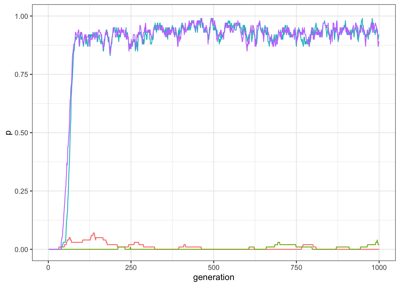

Figure 12.1: Frequency of traits in a world with four traits and pairwise compatibilities.

In the great majority of the runs, two out of the four traits diffuse in the population. We can check whether these are in fact one of the couple of compatible traits, having a look at the last line of the output produced by the simulation.

data_model[data_model$generation==1000, ]

## # A tibble: 4 x 3
##   trait generation     p
##   <chr>      <int> <dbl>
## 1 A           1000  0   
## 2 B           1000  0.02
## 3 C           1000  0.92
## 4 D           1000  0.89

Depending on random factors, the successful traits will be A and B or C and D. If you run the simulation again and again you would see that in around half of the simulations A and B are the successful traits, and in another half C and D are, and very few other possible cases with this “world” of compatibilities.

What happens if we change the world? We can run a new simulation where the traits A, B, and C are all compatible, but not D (remember, you can visualise the matrix of compatibilities by typing its name to be sure to have entered the compatibilities correctly).

my_world <- matrix(c(1,1,1,-1, 1,1,1,-1,1,1,1,-1,-1,-1,-1,1), nrow = 4, ncol = 4)
data_model <- traits_inter_dependence(N = 100, t_max = 1000, k = 10, 
                                      mu = 0.0005, p_death = 0.01, world = my_world)
plot_multiple_traits(data_model)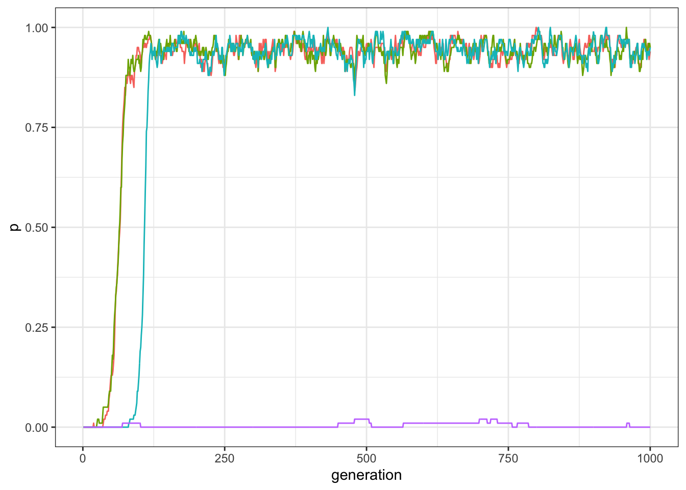

Figure 12.2: Frequency of traits in a world with four traits and three traits compatibile with each other, but not compatible with the fourth.

As expected, now three traits have high frequencies in the population, while one is unsuccessful. As before, you can check that the unsuccessful trait is actually D by inspecting manually the last line of the output.

Not surprisingly, if all traits are compatible, they all spread equally in the population.

my_world <- matrix(c(1,1,1,1,1,1,1,1,1,1,1,1,1,1,1,1), nrow = 4, ncol = 4)
data_model <- traits_inter_dependence(N = 100, t_max = 1000, k = 10, 
                                      mu = 0.0005, p_death = 0.01, world = my_world)
plot_multiple_traits(data_model)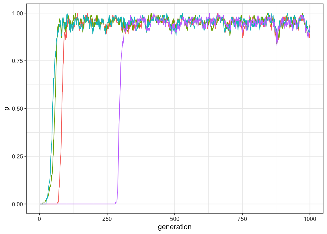

Figure 12.3: Frequency of traits in a world with four traits all compatibles with each other.

12.2 Many-traits model

Building the compatibility matrix by hand is not very practical, especially if we want to test our model with more traits. We will now extend the basic model above in order to be able to customise the maximum number of traits and to automatically generate the compatibility worlds.

M <- 7
gamma <- 0.5
my_world <- matrix( rep(1, M * M), nrow = M)
compatibilities <- sample(c(1, -1), choose(M, 2), prob = c(gamma, 1 - gamma), replace = TRUE) 
my_world[upper.tri(my_world)] <- compatibilities
my_world <- t(my_world)
my_world[upper.tri(my_world)] <- compatibilities

We have now two parameters we use to build the matrix: the maximum number of traits \(M\), and the probability that two traits are compatible with each other, \(\gamma\) (or gamma in the code). To build the matrix, we create a \(M\) by \(M\) matrix filled with \(1\)s, then a vector of compatibilities randomly generated with probability \(\gamma\) (the length of the vector is the number of entries above the main diagonal of the matrix, given by choose(M, 2)), and finally we copy the values the lower triangle to the upper triangle of the matrix (in practice, to make it symmetric, we copy it twice in the upper triangle, transposing the matrix after the first copy).

Have a look at the the matrix we just generated.

my_world

##      [,1] [,2] [,3] [,4] [,5] [,6] [,7]
## [1,]    1    1   -1   -1    1   -1    1
## [2,]    1    1   -1   -1   -1   -1    1
## [3,]   -1   -1    1    1   -1   -1   -1
## [4,]   -1   -1    1    1   -1    1    1
## [5,]    1   -1   -1   -1    1    1    1
## [6,]   -1   -1   -1    1    1    1   -1
## [7,]    1    1   -1    1    1   -1    1

The function to run the simulation is very similar to the previous one, once we account for the difference in how the compatibility matrix is created and for the two new parameters (\(M\) and \(\gamma\)) needed in the function call. Another difference is that the output data structure is a matrix and not a tibble. Since we want to be able to run the simulations with an arbitrary large number of traits, we need to speed up the computation, exactly in the same way as we did for the multiple traits model in chapter 7.

traits_inter_dependence_2 <- function(N, M, t_max, k, mu, p_death, gamma){
  output <- matrix(data = NA, nrow = t_max, ncol = M)
  
  # Initialise the traits' world
  world <- matrix( rep(1, M * M), nrow = M)
  compatibilities <- sample(c(1, -1), choose(M,2), prob = c(gamma, 1 - gamma), replace = TRUE) 
  world[upper.tri(world)] <- compatibilities
  world <- t(world)
  world[upper.tri(world)] <- compatibilities
  
  # Initialise the population
  population <- matrix(0, ncol = M, nrow = N)
  output[1, ] <- colSums(population) / N 
  
  for(t in 2:t_max){
    # Innovations
    innovators <- sample(c(TRUE, FALSE), N, prob = c(mu, 1 - mu), replace = TRUE) 
    innovations <- sample(1:M, sum(innovators), replace = TRUE)
    population[cbind(which(innovators == TRUE), innovations)] <- 1
    
    # Copying
    demonstrators <- sample(1:N, replace = TRUE)
    demonstrators_traits <- sample(1:M, N, replace = TRUE)

    for(i in 1:N){
      if(population[demonstrators[i], demonstrators_traits[i]]){
        compatibility_score <- sum(world[demonstrators_traits[i], which(population[i,]>0)])
        copy <- (1 / (1 + exp(-k*compatibility_score))) > runif(1)
        if(copy){
          population[i,demonstrators_traits[i]] <- 1
        }
      }
    }
    
    # Birth/death
    replace <- sample(c(TRUE, FALSE), N, prob = c(p_death, 1 - p_death), replace = TRUE)
    population[replace, ] <- 0
  
    # Write output
    output[t, ] <- colSums(population) / N
  }
  # Export data from function
  output
}  

We can now use the plot_multiple_traits_matrix() function (see chapter 7) to visualise the model results. Let’s have a look at what happens when we have 20 traits and an intermediate probability of compatibility.

data_model <- traits_inter_dependence_2(N = 100, M = 20, t_max = 2000, k = 10,
                                        mu = 0.001, p_death = 0.01, gamma = .5)
plot_multiple_traits_matrix(data_model)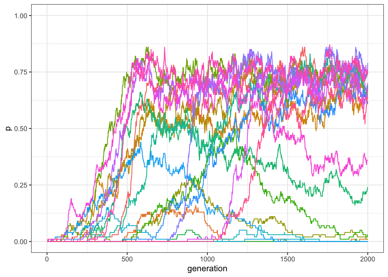

Figure 12.4: Frequency of traits in a world with 20 traits and compatiblity randomly generated. Each trait has 50% of probability of being compatible with each other trait.

The simulation generates a complex dynamic in which some of the traits spread in the population, while others do not. The success of a trait depends on its general compatibility with other traits but also on which traits are present at a certain point in time in the population. Some traits succeed to spread only after the traits they are compatible with have sufficiently spread in the population.

Let’s change \(\gamma\) to be \(1\), i.e. when all traits are compatible with each other.

data_model <- traits_inter_dependence_2(N = 100, M = 20, t_max = 2000, k = 10, 
                                        mu = 0.001, p_death = 0.01, gamma = 1)
plot_multiple_traits_matrix(data_model)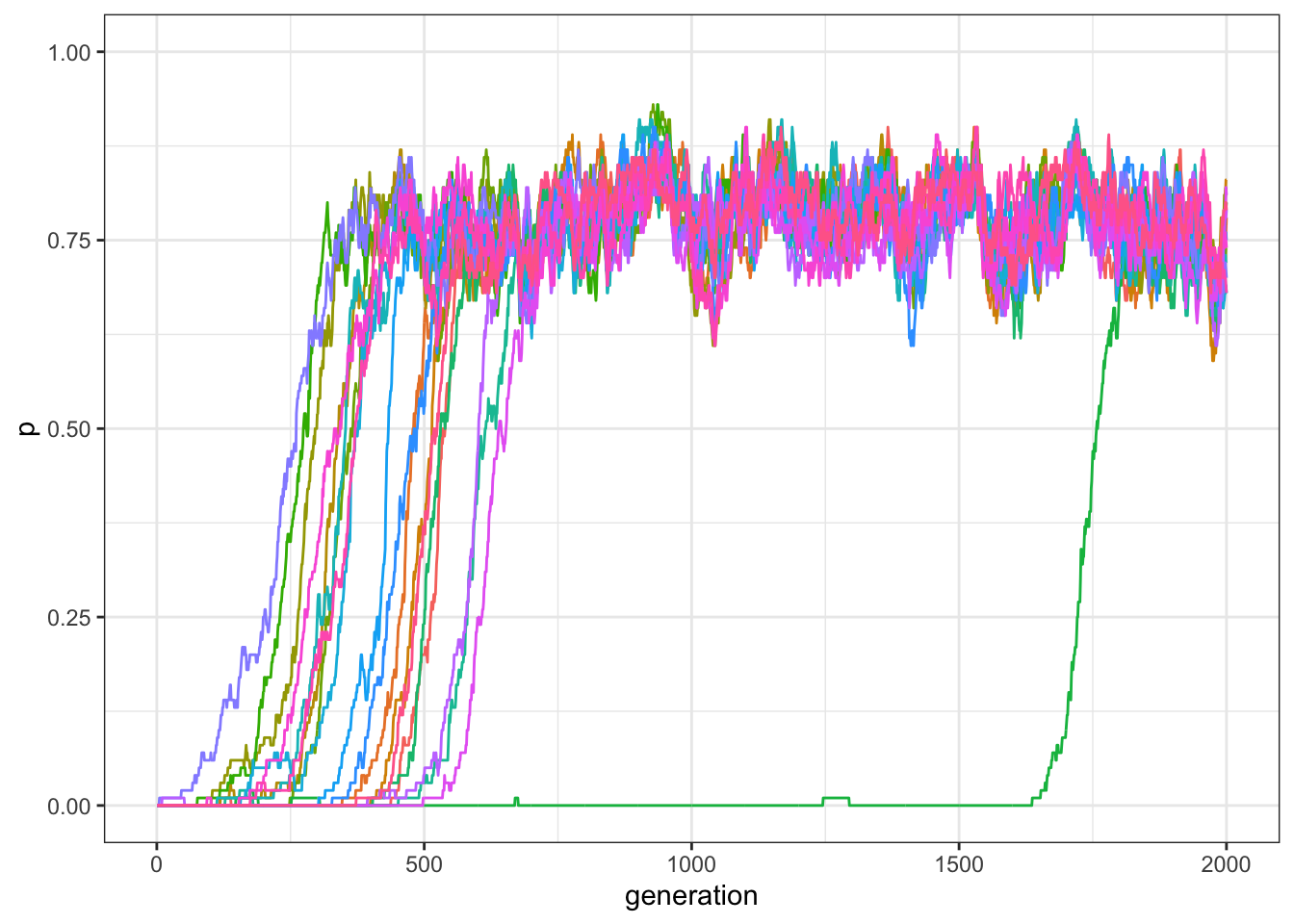

Figure 12.5: Frequency of traits in a world with 20 traits and compatiblity randomly generated. Each trait is compatible with all other traits.

As expected, all traits spread in the population.

We leave to the reader to explore further what drives the dynamic, especially in the interesting cases with intermediate values of \(\gamma\). In order to do this, we suggest to add further outputs to the function traits_inter_dependence_2(), such as the compatibility world generated by the simulation, or the actual composition of the population, perhaps only at the end, or every 100, or 500, time steps.

As an example, we can try to confirm the intuition that the final number of traits depends on the value of \(\gamma\): if it is more likely that traits are compatible with each other, we expect more traits to spread in the population. We can choose values of \(\gamma\) between \(0\) and \(1\) (with steps of \(0.1\)), and use a for cycle to run our function for each value. In fact, we are running another for cycle within the main one, as to have more runs for each value of \(\gamma\) (an alternative would be to rewrite the function traits_inter_dependence_2() to accept an additional argument that indicates the number of simulation repetitions, as we did in previous chapters).

Finally, we store the number of “successful” traits at the end of the simulation, that is, the traits that spread in at least half of the population (data_model[2000,]>.5).

r_max = 10
test_inter_dependence <- tibble(gamma = as.factor(rep(seq(0, 1, by = .1), r_max)), 
                                run = as.factor(rep(1:r_max, each = 11)), 
                                C = as.numeric(NA))
for(condition in seq(0, 1, by = .1)){
  for(r in 1:r_max) {
    data_model <- traits_inter_dependence_2(N = 100, M = 20, t_max = 2000, k = 10, 
                                            mu = 0.001, p_death = 0.01, gamma = condition)
    test_inter_dependence[test_inter_dependence$gamma == condition & 
                            test_inter_dependence$run == r, ]$C <- 
      sum(data_model[2000,]>.5)
  }
}

To plot the results, we combine boxplots and geom_jitter() so we can see the actual data points. (We introduced geom_jitter() in chapter 5.)

ggplot(data = test_inter_dependence, aes(x = gamma, y = C)) +
  geom_boxplot() +
  geom_jitter(width = 0.1, height = 0, alpha = 0.5) +
  theme_bw() +
  labs(x = "Average compatibility", y = "C (number of common traits)")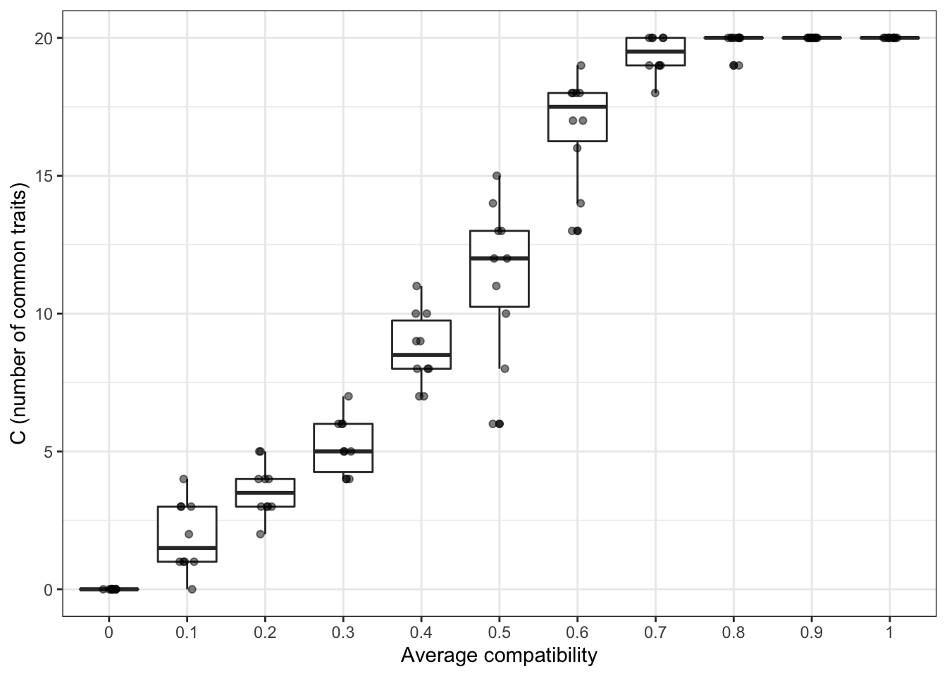

Figure 12.6: Increasing the probability of traits being compatible with each others produces bigger populations.

The results broadly confirm our intuitions. Interestingly, we do not need that all traits are compatible with each other to produce the outcome of all traits being successful. Already with \(\gamma=0.8\), all the 20 traits spread in more than half of the population in almost all runs of the simulation. Even with few incompatibilities, the “compatibility score” between observers and demonstrators is, given a sufficient number of compatible traits, a positive number, resulting in high probabilities to copy.

12.3 Summary of the model

Using simple models, we formalised the intuitive idea that cultural traits (can) have meaningful (for us) relationships with each other. When we decide whether to support a policy or not, to adopt a behaviour or not, or to participate in the latest fad, the decision may depend on how well the policy, the behaviour, or the fad fit with our pre-existing ideas. We used a simple rule for which traits can be compatible or incompatible with the other traits, and we showed that the success of traits depend on their compatibility. We also showed that, quite intuitively, populations where many traits are compatible with each other, will generate bigger cultures.

We also introduced a few new modelling devices, such as the logistic function, that transform unbounded positive and negative values into probabilities ranging from \(0\) to \(1\), and the ggplot geom geom_jitter(), which is useful to visualise overlapping data points.

12.4 Further readings

A broader treatment of models of cultural evolution where the outcomes depend on the relationships between traits, defined by the authors ‘cultural systems,’ is in Buskell, Enquist, and Jansson (2019). More complex relationships between traits, including the possibility that some trait will facilitate the appearance of new traits, generating cascade of innovations are explored in Enquist, Ghirlanda, and Eriksson (2011).