Chapter 10 Reproduction and transformation

To be considered ‘cultural,’ ideas, behaviours, and artefacts need to be sufficiently stable in time. The version of Little Red Riding Hood we heard now is part of a long cultural transmission chain that includes all the other versions of the tale because they all share enough features to be considered the same tale. Similarly, the lasagne I cooked yesterday are part of a long, intricate, chain of cultural transmission events, where all the products are stable enough that we can consider all of them as one cultural trait: lasagne. Boundaries are muddled for many traits: while some artefacts can be the exact replica of each other, no two identical lasagne exist. In any case, the question we explore in this chapter is: how does this stability is brought about? In the models so far, as much as in the majority of models in cultural evolution, we assumed that traits are copied from one (cultural) generation to another with enough fidelity to assure a relative stability. This is a useful assumption and, in many case, a good approximation of what happens in reality.

However, cultural traits can be stable not because they are copied with high-fidelity, but because, when passing from an individual to another, they are independently reconstructed in the same way or, another way to say it, they become similar to each other through a process of convergent transformation. Think about whistling. We do learn to whistle from each other through a process of cultural transmission (we want to reproduce what others do), but the configuration of the muscles in the mouth is not something that we copy directly. Still, there are few ways to effectively whistle, so that we likely end up with the same - or similar - configuration. (Notice we can also actually copy the exact configuration and, indeed, there are specialised whistling techniques for which it is required. As we will mention again later, copying and reconstructing are not two alternative processes, but they both concur to cultural evolution.)

Evolutionary psychologists and some anthropologists emphasise how certain cultural traditions are similar in many societies, such as supernatural beliefs, types of musics, or what people find or not disgusting. These similarities do not need to be produced by genetically encoded preferences, but it suffices that some general tendencies make more likely that people everywhere will converge on these quasi-universal forms. A psychological tendency to interpret the behaviour of an entity as intentional (even if this entity is an inanimate object) could give rise to similarity in supernatural beliefs, as much as the physical property of the mouth give rise to similarity in how people whistle everywhere.

10.1 Copying and selection

To have a better grasp of the consequence of this idea we can, as usual, try to model a very simple case, where cultural stability can be obtained with a process of copying and selection of a model, as we did in many of the previous chapters, or with convergent transformation, where individuals are not very good at copying, or at selecting models, but they tend to transform the trait in the same way.

Let’s imagine a population with a single trait, a continuous trait \(P\), that can have values between 0 and 1. At the beginning of the simulations, \(P\) is uniformly distributed in the population. Let’s say the optimal value of \(P\) is \(1\) (this is convenient for the code, but the exact value is not important). You can think to \(P\) as, for example, how sharp is a knife: the sharper the better.

library(tidyverse)
N <- 1000
population <- tibble(P = runif(N))

Now, we can write the familiar function where individuals copy the trait from the previous generation with one of the biases we explored earlier in the book. In Chapter 3, for example, we showed how a direct bias for one of two discrete cultural traits could make it spread and go to fixation. We can do something similar here, with the difference that the trait is continuous and the bias needs to be a preference for traits close to the optimal value. (Notice the code would be equivalent - and we would obtain the same effect of convergence to optimal value - thinking in terms of other methods of cultural selection, e.g. an indirect bias towards successful demonstrators, that are successful as they have a \(P\) close to the optimal).

reproduction <- function(N, t_max, r_max, mu) {
  output <- tibble(generation = rep(1:t_max, r_max), 
                   p = as.numeric(rep(NA, t_max * r_max)), 
                   run = as.factor(rep(1:r_max, each = t_max)))
  for (r in 1:r_max) {
    # Create first generation
    population <- tibble(P = runif(N))
    
    # Add first generation's p for run r
    output[output$generation == 1 & output$run == r, ]$p <- sum(population$P) / N 
    
    for (t in 2:t_max) {
      # Copy individuals to previous_population tibble
      previous_population <- population 
      
      # Select a pair of demonstrator for each individual
      demonstrators <- tibble(P1 = sample(previous_population$P, N, replace = TRUE), 
                              P2 = sample(previous_population$P, N, replace = TRUE))
      
      # Copy the one with the trait value closer to 1
      copy <- pmax(demonstrators$P1, demonstrators$P2)
      
      # Add mutation
      population$P <- copy + runif(N, -mu, +mu)
      
      # Keep the  traits' value in the boundaries [0,1]
      population$P[population$P > 1] <- 1
      population$P[population$P < 0] <- 0
      
      # Get p and put it into output slot for this generation t and run r
      output[output$generation == t & output$run == r, ]$p <- 
        sum(population$P) / N 
    }
  }
  # Export data from function
  output 
}

The function is similar to what we have already done several times. Let’s have a look at the few differences. First, we find again the parameter \(\mu\), as done in various previous chapters. Similarly, it implements here the error in copying: with respect to the \(P\) of the demonstrator chosen, the new trait will vary of maximum of \(\mu\), through the instruction runif(N, -mu, +mu). The two following lines just keep the traits in the boundaries between \(0\) and \(1\). The second difference is in the selection of the trait to copy. Here each individual sample two traits (or demonstrators) from the previous generation, and simply copies the one with the trait closer to the optimal value of \(1\).

We can now run the simulation, and plot it with a slightly modified function plot_multiple_runs_p() (we just need to change the label for y-axis). We use a low value for the copying error, such as \(\mu=0.05\).

plot_multiple_runs_p <- function(data_model) {
  ggplot(data = data_model, aes(y = p, x = generation)) +
    geom_line(aes(colour = run)) +
    stat_summary(fun = mean, geom = "line", size = 1) +
    ylim(c(0, 1)) +
    theme_bw() +
    labs(y = "p (average value of P)")
}

data_model <- reproduction(N = 1000, t_max = 20, r_max = 5, mu = 0.05)
plot_multiple_runs_p(data_model)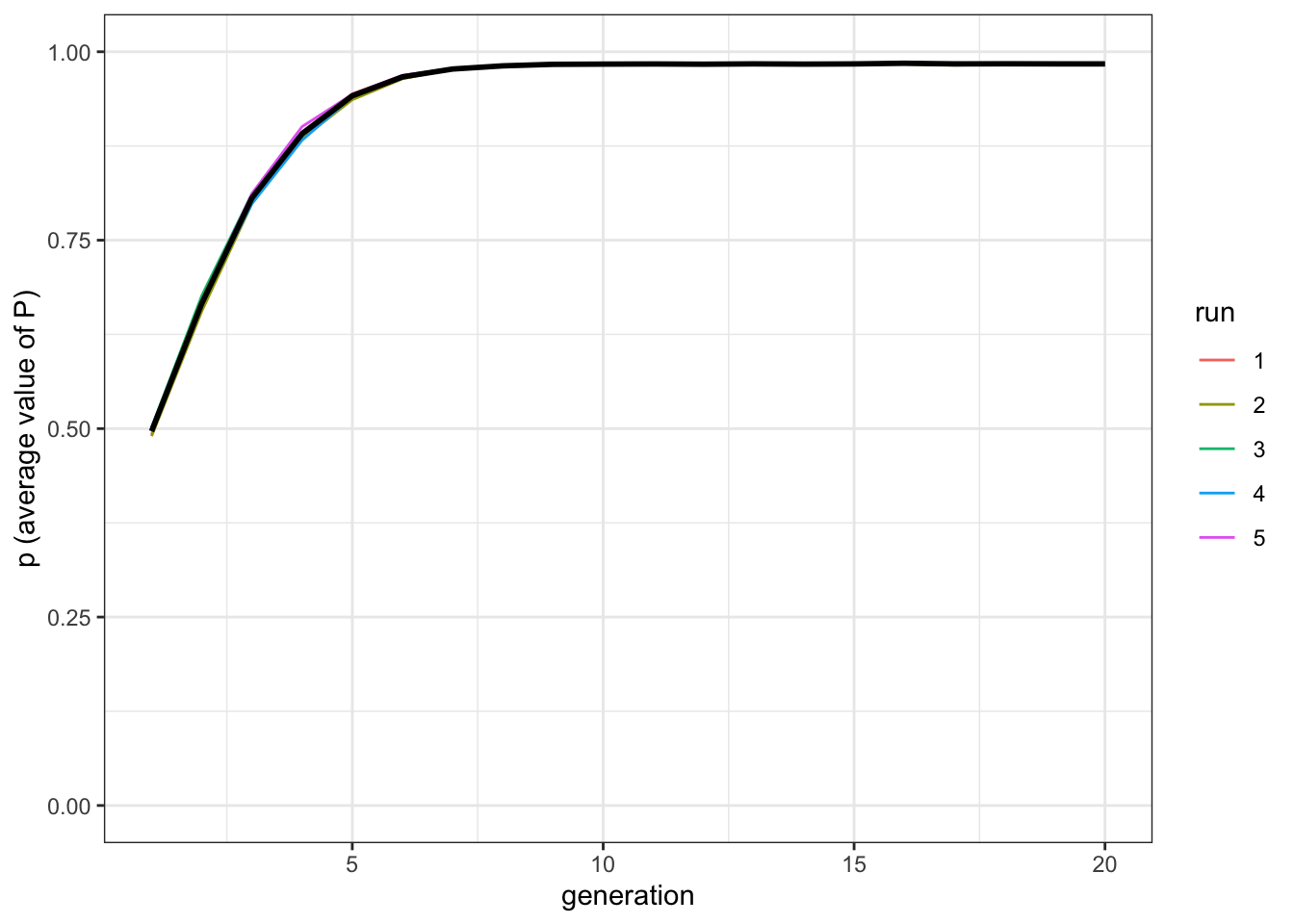

Figure 10.1: The populations reach the optimal trait value with cultural selection.

Even with a weak form of selection (sampling two traits and choosing the better one) the population converges on the optimal value quickly, in only around ten cultural generations.

10.2 Convergent transformation

Now we can write another function where convergent transformation produces the same effect.

transformation <- function(N, t_max, r_max) {
  output <- tibble(generation = rep(1:t_max, r_max), 
                   p = as.numeric(rep(NA, t_max * r_max)), 
                   run = as.factor(rep(1:r_max, each = t_max)))
  
  for (r in 1:r_max) {
    # Create first generation
    population <- tibble(P = runif(N))
    
    # Add first generation's p for run r
    output[output$generation == 1 & output$run == r, ]$p <- sum(population$P) / N 
    
    for (t in 2:t_max) {
       # Copy individuals to previous_population tibble
      previous_population <- population
      
      # Only one demonstrator is selected at random for each individual
      demonstrators <- tibble(P = sample(previous_population$P, N, replace = TRUE))
      
      # The new P is in between the demonstrator's value and 1
      population$P <- demonstrators$P + runif(N, max = 1 - demonstrators$P)
      
      # Get p and put it into output slot for this generation t and run r
      output[output$generation == t & output$run == r, ]$p <- sum(population$P) / N 
    }
  }
  # Export data from function
  output 
}

There is only a line we need to pay attention to: the values of \(P\) of the new generation are calculated as demonstrators$P + runif(N, max = 1-demonstrators$P). This means that the individuals of the new population copy the old generation, but they are not particularly good. They take a value of \(P\) randomly drawn between the value of the demonstrator and the optimal \(P=1\). Thus, if they attempt to copy a demonstrator with \(P=0.1\), their ‘error’ can be as large as 0.9. While modifications can be big, they are all in the same direction, contributing to increase \(P\). Let’s run the simulations.

data_model <- transformation(N = 1000, t_max = 20, r_max = 5)
plot_multiple_runs_p(data_model)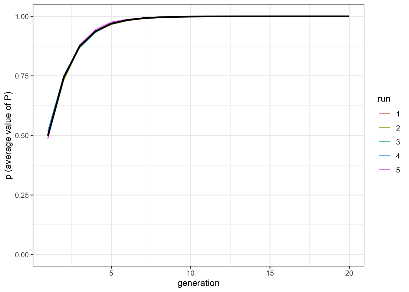

Figure 10.2: The population reach the optimal trait value when transformations converge towards the optimal value.

As the transformations tend to all converge in the same direction, the results are equivalent to the previous model. It does not matter when exactly the population reaches stability at \(P=1\), as this depends on the specific implementation choices, for example the strength of cultural selection in the first model, or how big can be the ‘jump’ of the transformation in the second model (you can try to modify those by yourself).

When we see cultural traits in real life, we are observing systems in a state analogous to what happens on the right side of the two plots, where individuals reproduce traits one similar to the other. As we touched earlier in the chapter, both faithful copying coupled with selection and transformation can be important for culture, and their importance can depend from the specific features we are interested to track, or from the cultural domain. As we have just shown, however, the spread of the traits in the population looks similar in both cases. Are there ways to distinguish the relative importance of the two processes?

10.3 Emergent similarity

One possibility is to track how similar are the traits that the observers reproduce, with respect to the traits they use as a starting point. If reproduction is the driving force, they should be fairly similar and the measure should be always the same, as the distance between the trait produced and the trait copied is fixed, and given by the parameter \(\mu\). If transformation is the driving force, instead, we should expect similarity being lower when traits are far from the optimal value (i.e. at the beginning of the simulations), and higher when traits are close to the optimal value.

We can rewrite the reproduction() and transformation() functions adding as a further output this measure of similarity, that is, how distant are the traits that the new generation show versus the traits that they had copied from the previous. We thus add a variable d (as in ‘distance’) in our output tibble, and we calculate this value at the end of each generation as sum(abs(population$P - copy)) / N.

reproduction <- function(N, t_max, r_max, mu) {
  output <- tibble(generation = rep(1:t_max, r_max), 
                   p = as.numeric(rep(NA, t_max * r_max)), 
                   run = as.factor(rep(1:r_max, each = t_max)), 
                   d = as.numeric(rep(NA, t_max * r_max)))
  for (r in 1:r_max) {
    # Create first generation
    population <- tibble(P = runif(N))
    
    # Add first generation's p for run r
    output[output$generation == 1 & output$run == r, ]$p <- sum(population$P) / N 
    
    for (t in 2:t_max) {
      # Copy individuals to previous_population tibble
      previous_population <- population
      
      demonstrators <- tibble(P1 = sample(previous_population$P, N, replace = TRUE), 
                              P2 = sample(previous_population$P, N, replace = TRUE))
      
      copy <- pmax(demonstrators$P1, demonstrators$P2)

      population$P <- copy + runif(N, -mu, +mu)
      population$P[population$P > 1] <- 1
      population$P[population$P < 0] <- 0
      
      # Output:
      output[output$generation == t & output$run == r, ]$p <- sum(population$P) / N 
      output[output$generation == t & output$run == r, ]$d <- sum(abs(population$P - copy)) / N
    }
  }
  # Export data from function
  output 
}

We do the same for the transformation() function, and we can run again both simulations.

transformation <- function(N, t_max, r_max) {
  output <- tibble(generation = rep(1:t_max, r_max), 
                   p = as.numeric(rep(NA, t_max * r_max)), 
                   run = as.factor(rep(1:r_max, each = t_max)), 
                   d = as.numeric(rep(NA, t_max * r_max)))
  
  for (r in 1:r_max) {
    # Create first generation
    population <- tibble(P = runif(N))
    
    # Add first generation's p for run r
    output[output$generation == 1 & output$run == r, ]$p <- sum(population$P) / N 
    
    for (t in 2:t_max) {
      # Copy individuals to previous_population tibble
      previous_population <- population 
      
      demonstrators <- tibble(P = sample(previous_population$P, N, replace = TRUE))
      
      population$P <- demonstrators$P + runif(N, max = 1-demonstrators$P)
      
      # Output
      output[output$generation == t & output$run == r, ]$p <- sum(population$P) / N 
      output[output$generation == t & output$run == r, ]$d <- sum(abs(population$P - demonstrators$P)) / N
    }
  }
  # Export data from function
  output 
}

data_model_reproduction <- reproduction(N = 1000, t_max = 20, r_max = 5, mu = 0.05)
data_model_transformation <- transformation(N = 1000, t_max = 20, r_max = 5)

We already know the results with respect to the value of \(P\), but now we are interested in comparing if and how the values for \(d\) change in time in the two conditions. For this, we write an ad hoc plotting function, that takes the data from the two outputs and plot them in the same graph. Notice the na.omit() function in the first line: the data on d is NA for the first generation, because there is no previous generation from which to take the measure, so we want to exclude it from our plot, and start from generation number 2. For this reason, all the other values are rescaled and, in particular, the variable generation starts from 2.

data_to_plot <- tibble(distance = c(na.omit(data_model_reproduction$d), 
                                    na.omit(data_model_transformation$d)), 
                       condition = rep(c("reproduction", "transformation"), each = 95),
                       generation = rep(2:20,10),
                       run = as.factor(rep(1:10, each = 19)))
ggplot(data = data_to_plot, aes(y = distance, x = generation, group = run, color = condition)) +
  geom_line() +   
  geom_point() +
  theme_bw() +
  labs(y = "d (average distance observer/demonstrator)")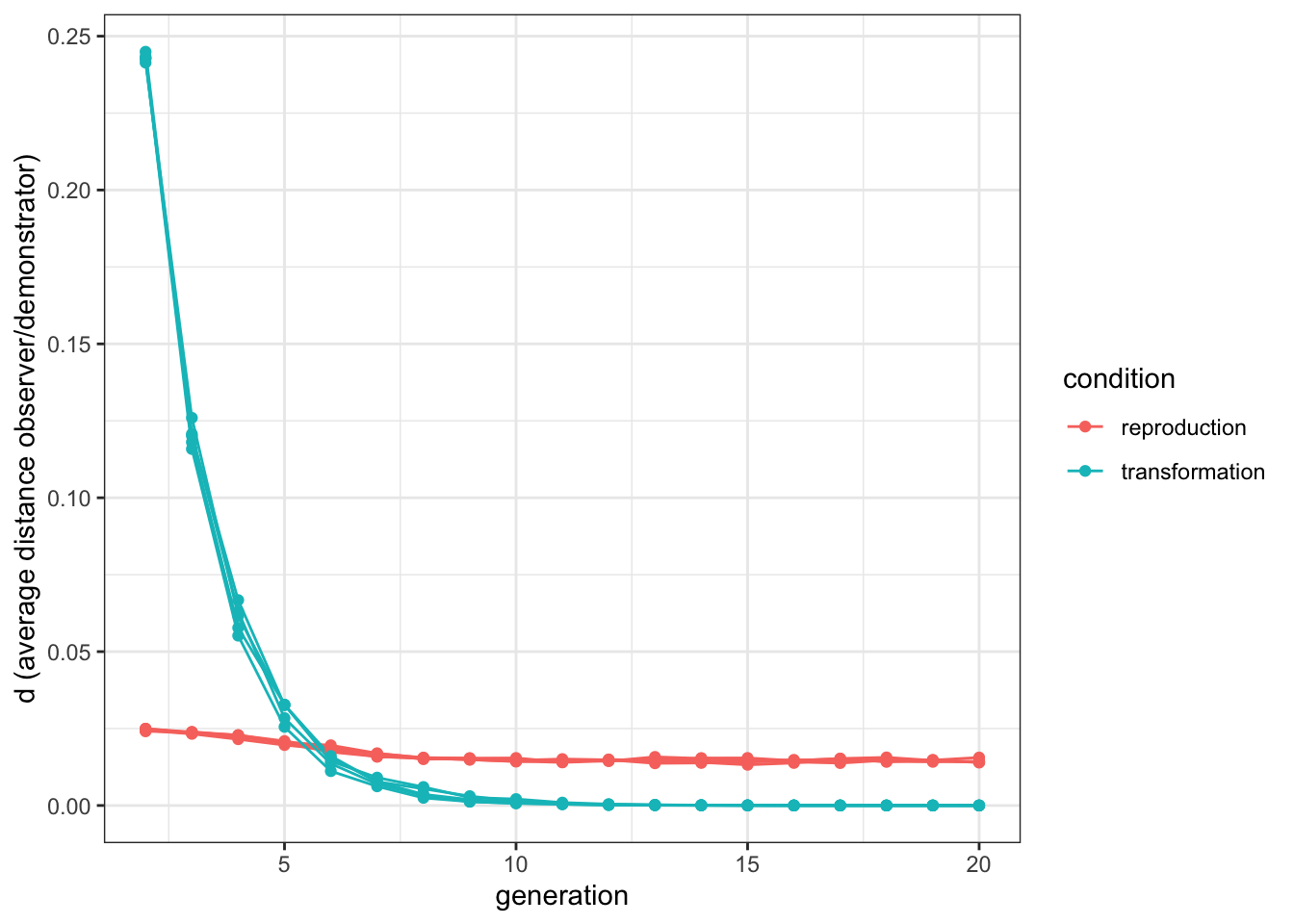

Figure 10.3: When convergent transformation is the driving force, the similarity between original and copied items starts high and decreases with time. When cultural selection is the driving force, the similarity is constant.

As predicted, in the ‘transformation’ condition distance is higher at the beginning of the simulation, and reaches zero when all individuals have the optimal value. In the “reproduction” condition, instead, the distance is approximately constant. In fact, it slightly decreases after the first few generations. This is due to the fact that at the beginning, with \(P\) randomly distributed in the population, the mutation is effectively drawn between \(P-\mu\) and \(P+\mu\), but after a while, when demonstrators have a value close to the optimal \(P=1\), the mutation is only drawn in \(P-\mu\), as values of \(P\) higher than \(1\) are not allowed.

10.4 Cultural fitness

Another way to look at the difference between the two conditions, focusing on the process of selection, is to look at the ‘cultural fitness’ of the individuals in the population. More in detail, one can look at how this metric covaries with how good they actually are, as given by their value of \(P\). We can define \(W\), a measure of cultural fitness, as the number of “cultural offspring” that the individual \(i\) has in the next generation. If individual \(i\) has been copied by, say, four individuals, its fitness will be \(W_i=4\).

If individuals, or their traits, are selected, as happens in the “reproduction” condition, we expect that individuals with higher values of \(P\) have more cultural offspring, thus, that to higher \(P\)s correspond higher \(W\)s. We expect, in other words, the covariance between \(W\) and \(P\) being positive i.e. \(cov(W,P)>0\). On the other hand, in the condition “transformation” there is no selection, and there are no reasons why an individual with higher \(P\) produces more cultural offspring. In this case, the covariance should be zero, i.e. \(cov(W,P)=0\).

To calculate cultural fitness, and how it covaries with \(P\), we need to modify again our functions. Let’s start, as before, with reproduction():

reproduction <- function(N, t_max, r_max, mu) {
  output <- tibble(generation = rep(1:t_max, r_max), 
                   p = as.numeric(rep(NA, t_max * r_max)), 
                   run = as.factor(rep(1:r_max, each = t_max)), 
                   cov_W_P = as.numeric(rep(NA, t_max * r_max)))
  for (r in 1:r_max) {
    # Create first generation
    population <- tibble(P = runif(N))
    
    # Add first generation's p for run r
    output[output$generation == 1 & output$run == r, ]$p <- sum(population$P) / N 
    
    for (t in 2:t_max) {
      # Copy individuals to previous_population tibble
      previous_population <- population 
      
      # Sample the demonstrators using their indexes
      demonstrators <- cbind(sample(N, N, replace = TRUE), sample(N, N, replace = TRUE))
      # Retrieve their traits from the indexes 
      copy <- max.col(cbind(previous_population[demonstrators[,1],], 
                            previous_population[demonstrators[,2],]))
      # Save the demonstrators
      demonstrators <- demonstrators[cbind(1 : N, copy)]
      fitness <- tabulate(demonstrators, N) 

      population$P <- previous_population[demonstrators,]$P + runif(N, -mu, +mu)
      population$P[population$P > 1] <- 1
      population$P[population$P < 0] <- 0
      
      # Output
      output[output$generation == t & output$run == r, ]$p <- 
        sum(population$P) / N 
      output[output$generation == t & output$run == r, ]$cov_W_P <- 
        cov(fitness, previous_population$P) 
    }
  }
  # Export data from function
  output 
}

The function produces the usual output, but in a different way. To measure \(W\), we need to know the actual individuals that are copied, not only their \(P\) values, as we were doing previously. For this reason, the sampling of the demonstrators is done on their indexes with the instruction sample(N, N, replace = TRUE). Then, the indexes are used to retrieve their \(P\), in the two following lines. Finally, we count how many times each index, that is, each individual, is used as demonstrator, using the function tabulate(), introduced in Chapter 7.

Now we need to do the same for transformation():

transformation <- function(N, t_max, r_max) {
  output <- tibble(generation = rep(1:t_max, r_max), 
                   p = as.numeric(rep(NA, t_max * r_max)), 
                   run = as.factor(rep(1:r_max, each = t_max)), 
                   cov_W_P = as.numeric(rep(NA, t_max * r_max)))
  for (r in 1:r_max) {
    # Create first generation
    population <- tibble(P = runif(N))
    
    # Add first generation's p for run r
    output[output$generation == 1 & output$run == r, ]$p <- sum(population$P) / N 
    for (t in 2:t_max) {
      # Copy individuals to previous_population tibble
      previous_population <- population 
      
      # Choose demonstrators and calcualte  their fitness
      demonstrators <- sample(N, N, replace = TRUE)
      fitness <- tabulate(demonstrators, N) 

      population$P <- previous_population[demonstrators,]$P + 
        runif(N, max = 1 - previous_population[demonstrators,]$P)
      
      # Output
      output[output$generation == t & output$run == r, ]$p <- sum(population$P) / N 
      output[output$generation == t & output$run == r, ]$cov_W_P <- cov(fitness,previous_population$P)
    }
  }
  # Export data from function
  output 
}

The logic is exactly the same, only we do not need to use the indexes to retrieve the \(P\) values, as they are not needed to choose demonstrators. At this point, as before, we can run the simulations in the two conditions, and plot the results (the code for the plot is also the same, only the label for the y-axes changes).

data_model_reproduction <- reproduction(N = 1000, t_max = 20, r_max = 5, mu = 0.05)
data_model_transformation <- transformation(N = 1000, t_max = 20, r_max = 5)

data_to_plot <- tibble(covariance = c(na.omit(data_model_reproduction$cov_W_P), 
                                      na.omit(data_model_transformation$cov_W_P)), 
                       condition = rep(c("reproduction", "transformation"), each = 95),
                       generation = rep(2:20,10),
                       run = as.factor(rep(1:10, each = 19)))
ggplot(data = data_to_plot, aes(y = covariance, x = generation, 
                                group = run, color = condition)) +
  geom_line() +   
  geom_point() +
  theme_bw() +
  labs(y = "covariance between cultural fitness and P")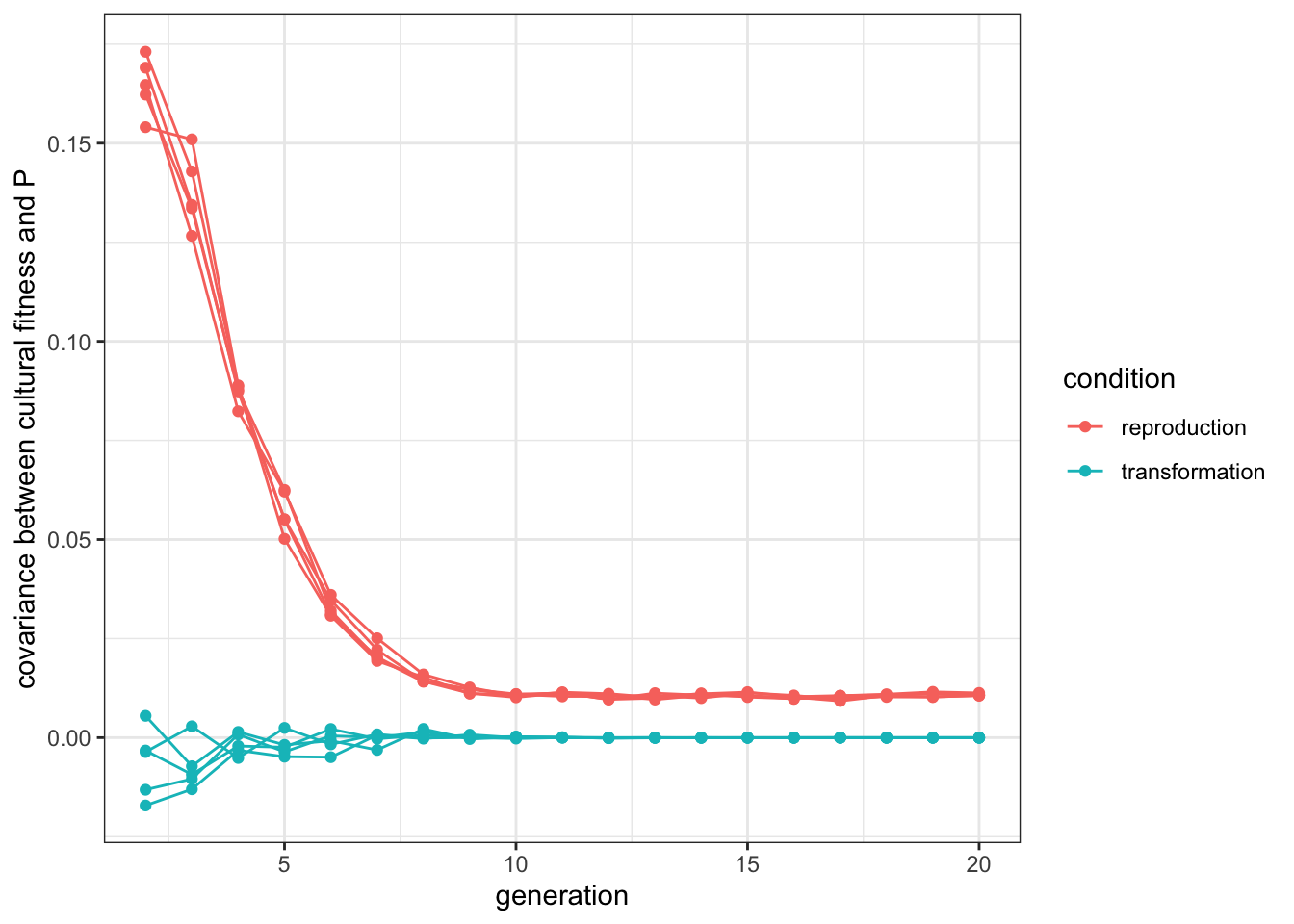

Figure 10.4: When cultural selection is the driving force, better cultural items are more likely to be copied (until the population converges to optimal values). When convergent transformation is the driving force, there is no relationship between quality and cultural success.

In the ‘reproduction’ condition, the covariance is indeed positive, and decreases gradually close to zero, when all the individuals converge to \(P=1\), as there is no more variation on which selection can act. Notice it does not reach zero, as mutation keeps some variation, and individuals that muted to lower \(P\)s are less likely to be selected. As expected, the covariance is equal to zero in the ‘transformation’ condition. This is hardly a surprising result as demonstrators are selected fully at random in the model, but it is important to compare this with what happens with empirical data of real cultural dynamics, where we can be able to distinguish different underlying stabilising forces.

10.5 Summary of the model

Cultural traditions can survive intact through long and wide transmission chains because cultural traits are copied faithfully, because some of them are copied more than others (cultural selection), and because everybody involved in the episodes of transmission tend to reproduce them in a similar way. All these forces are likely to be important, to a various degree, in different domains and for different features of cultural traits. While in the rest of the book we have focused on copying and selection, in this chapter we have considered transformation. We have shown that both copying plus selection and convergent transformation create stable cultural systems, where all individuals in the population converge on similar cultural traits. We also explored how these forces can be distinguished. One possible way is to chart the similarity between the cultural traits observed and the cultural traits reproduces: in the case of transformation depends on the specific feature of the traits (the closer to the end-point of the convergence, the higher the similarity), whereas for reproduction we should expect similarity to be constant, depending on how, generally, copying is precise. Another way is to detect whether demonstrators with certain traits (or certain features of a trait) are copied more: this is the sign of selection, that characterised our ‘reproduction’ model, but not the ‘transformation’ one.

10.6 Further readings

The model comparing reproduction and transformation is a simplified version of the model described in Acerbi et al. (2019). The analysis to detect signs (similarity and cultural fitness) of the two forces are inspired also by the application of the Price Equation to cultural evolution in Nettle (2020). An early account of the importance of convergent transformation (‘cultural attraction’) in cultural evolution is Sperber (1997). A discussion of the relative importance of transformation and reproduction in cultural evolution, and of the necessity to consider both is Acerbi and Mesoudi (2015).