Chapter 9 Rogers’ Paradox: A Solution
In the previous chapter we saw how social learning does not increase the mean fitness of a population relative to a population entirely made up of individual learners, at least in a changing environment. This is colloquially known as Rogers’ paradox, after Alan Rogers’ model which originally showed this. It is a ‘paradox’ because it holds even though social learning is less costly than individual learning, and social learning is often argued to underpin our species’ ecological success. The paradox occurs because social learning is frequency dependent: when environments change, the success of social learning depends on there being individual learners around to copy. Otherwise social learners are left copying each others’ outdated behaviour.
Several subsequent models have explored ‘solutions’ to Rogers’ paradox. These involve relaxing the obviously unrealistic assumptions. One of these is that individuals in the model come in one of two fixed types: social learners (who always learn socially), and individual learners (who always learn individually). This is obviously unrealistic. Most organisms that can learn individually can also learn socially, and the two capacities likely rely on the same underlying mechanisms (e.g. associative learning, see e.g. Heyes (2012)).
9.1 Modelling critical social learners
To explore how a mixed learning strategy would compete with pure strategies (only social or only individual learning), Enquist, Eriksson, and Ghirlanda (2007) added another type of individual to Rogers’ model: a critical social learner. These individuals first try social learning, and if the result is unsatisfactory, they then try individual learning.
The following function modifies the rogers_model() function from the last chapter to include critical learners. We need to change the code in a few places, but the modifications should be all easy to understand at this point. To start with, in the output tibble, we need to track the proportion of individual learners (before they were simply the individuals that were not social learners) and of the proportion of the individuals adopting the new strategy, critical social learning. We have now two more variables for this: p_IL and p_CL. Next, we need to add a learning routine for critical learners. This involves repeating the social learning code originally written for the social learners. We then apply the individual learning code to those critical learners who copied the incorrect behaviour, i.e. if their behaviour is different from E (this makes them ‘unsatisfied’). To make it easier to follow, we now insert the fitness updates into the learning section. This is because only those critical learners who are unsatisfied will suffer the costs of individual learning. If we left it to afterwards, it’s easy to lose track of who is paying what fitness cost.
Reproduction and mutation are changed to account for the three learning strategies. We now need to get the relative fitness of social and individual learners, and then reproduce based on those fitnesses. Individuals left over become critical learners. We could calculate the relative fitness of critical learners, but it’s not really necessary given that the proportion of critical learners will always be 1 minus the proportion of social and individual learners. Similarly, mutation now needs to specify that individuals can mutate into either of the two other learning strategies. We assume this mutation is unbiased, and mutation is equally likely to result in the two other strategies. Notice the use of the function sample() when we set the learning strategies of the new population. So far we used it for binary choices, now we are using it with three elements (c("individual", "social", "critical") and three probabilities (prob = c(fitness_IL, fitness_SL, 1 - (fitness_SL + fitness_IL))).
library(tidyverse)

rogers_model2 <- function(N, t_max, r_max, w = 1, b = 0.5, c, s = 0, mu, p, u) {

  # Check parameters to avoid negative fitnesses
  if (b * (1 + c) > 1 || b * (1 + s) > 1) {
    stop("Invalid parameter values: ensure b*(1+c) < 1 and b*(1+s) < 1")
  }

  # Create output tibble
  output <- tibble(generation = rep(1:t_max, r_max),
                   run = as.factor(rep(1:r_max, each = t_max)),
                   p_SL = as.numeric(rep(NA, t_max * r_max)),
                   p_IL = as.numeric(rep(NA, t_max * r_max)),
                   p_CL = as.numeric(rep(NA, t_max * r_max)),
                   W = as.numeric(rep(NA, t_max * r_max)))

  for (r in 1:r_max) {

    # Create a population of individuals
    population <- tibble(learning = rep("individual", N),
                         behaviour = rep(NA, N), fitness = rep(NA, N))

    # Initialise the environment
    E <- 0

    for (t in 1:t_max) {

      # Now we integrate fitnesses into the learning stage
      population$fitness <- w

      # 1. Social learning
      if (sum(population$learning == "social") > 0) {
        # Subtract cost b*s from fitness of social learners
        population$fitness[population$learning == "social"] <-
          population$fitness[population$learning == "social"] - b*s
        # Update behaviour
        population$behaviour[population$learning == "social"] <-
          sample(previous_population$behaviour, sum(population$learning == "social"), replace = TRUE)

      }

      # 2. Individual learning
      # Subtract cost b*c from fitness of individual learners
      population$fitness[population$learning == "individual"] <-
        population$fitness[population$learning == "individual"] - b*c
      # Update behaviour
      learn_correct <- sample(c(TRUE, FALSE), N, prob = c(p, 1 - p), replace = TRUE)
      population$behaviour[learn_correct & population$learning == "individual"] <- E
      population$behaviour[!learn_correct & population$learning == "individual"] <- E - 1


      # 3. Critical social learning
      if (sum(population$learning == "critical") > 0) {

        # Subtract b*s from fitness of socially learning critical learners
        population$fitness[population$learning == "critical"] <-
          population$fitness[population$learning == "critical"] - b*s

        # First critical learners socially learn
        population$behaviour[population$learning == "critical"] <-
          sample(previous_population$behaviour,
                 sum(population$learning == "critical"), replace = TRUE)

        # Subtract b*c from fitness of individually learning critical learners
        population$fitness[population$learning == "critical" & population$behaviour != E] <-
          population$fitness[population$learning == "critical" & population$behaviour != E] - b*c

        # Individual learning for those critical learners who did not copy correct behaviour
        population$behaviour[learn_correct & population$learning == "critical" & population$behaviour != E] <- E
        population$behaviour[!learn_correct & population$learning == "critical" & population$behaviour != E] <- E - 1
      }

      # 4. Calculate fitnesses (now only need to do the b bonus or penalty)
      population$fitness[population$behaviour == E] <-
        population$fitness[population$behaviour == E] + b
      population$fitness[population$behaviour != E] <-
        population$fitness[population$behaviour != E] - b

      # 5. store population characteristics in output
      output[output$generation == t & output$run == r, ]$p_SL <-
        mean(population$learning == "social")
      output[output$generation == t & output$run == r, ]$p_IL <-
        mean(population$learning == "individual")
      output[output$generation == t & output$run == r, ]$p_CL <-
        mean(population$learning == "critical")
      output[output$generation == t & output$run == r, ]$W <-
        mean(population$fitness)

      # 6. Reproduction
      previous_population <- population
      population$behaviour <- NA
      population$fitness <- NA

      # Individual learners
      if (sum(previous_population$learning == "individual") > 0) {
        fitness_IL <- sum(previous_population$fitness[previous_population$learning == "individual"]) /
          sum(previous_population$fitness)
      } else {
        fitness_IL <- 0
      }

      # Social learners
      if (sum(previous_population$learning == "social") > 0) {
        fitness_SL <- sum(previous_population$fitness[previous_population$learning == "social"]) /
          sum(previous_population$fitness)
      } else {
        fitness_SL <- 0
      }

      population$learning <- sample(c("individual", "social", "critical"), size = N,
             prob = c(fitness_IL, fitness_SL, 1 - (fitness_SL + fitness_IL)), replace = TRUE)

      mutation <- sample(c(TRUE, FALSE), N, prob = c(mu, 1 - mu), replace = TRUE)

      previous_population2 <- population

      population$learning[mutation & previous_population2$learning == "individual"] <-
        sample(c("critical", "social"),
               sum(mutation & previous_population2$learning == "individual"),
               prob = c(0.5, 0.5), replace = TRUE)

      population$learning[mutation & previous_population2$learning == "social"] <-
        sample(c("critical", "individual"),
               sum(mutation & previous_population2$learning == "social"),
               prob = c(0.5, 0.5), replace = TRUE)

      population$learning[mutation & previous_population2$learning == "critical"] <-
        sample(c("individual", "social"),
               sum(mutation & previous_population2$learning == "critical"),
               prob = c(0.5, 0.5), replace = TRUE)

      # 7. Potential environmental change
      if (runif(1) < u) E <- E + 1
    }
  }
  # Export data from function
  output
}
Now we can run rogers_model2(), with the same parameter values as we initially ran rogers_model() in the last chapter.
data_model <- rogers_model2(N = 1000, t_max = 200, r_max = 10, c = 0.9, mu = 0.01, p = 1, u = 0.2)As before, it’s difficult to see what’s happening unless we plot the data. The following function plot_prop() now plots the proportion of all three learning strategies. To do this we need to convert our wide data_model tibble (where each strategy is in a different column) to long format (where all proportions are in a single column, and a new column indexes the strategy). To do this we use pivot_longer(), similarly to what we did in Chapter 7. For visualisation purposes, we also rename the variables that keep track of the frequencies of the strategies (p_IL, p_SL, p_CL) with full words. For this plot, we only visualise the averages of all runs with the stat_summary() function.
plot_prop <- function(data_model) {

  names(data_model)[3:5] <- c("social", "individual", "critical")
  data_model_long <- pivot_longer(data_model, -c(W, generation, run),
                                  names_to = "learning",
                                  values_to = "proportion")

  ggplot(data = data_model_long, aes(y = proportion, x = generation, colour = learning)) +
    stat_summary(fun = mean, geom = "line", size = 1) +
    ylim(c(0, 1)) +
    theme_bw() +
    labs(y = "proportion of learners")
}

plot_prop(data_model)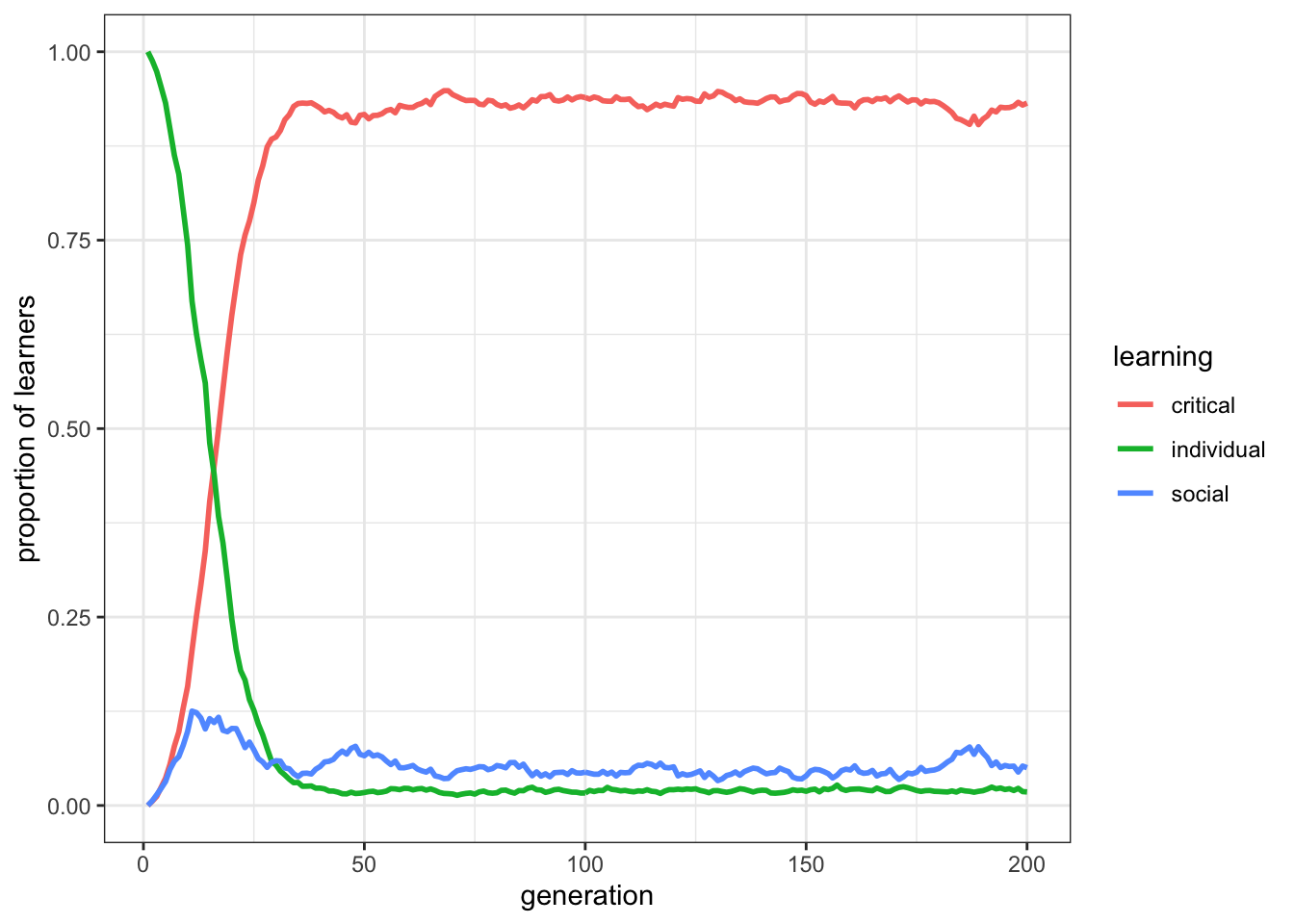
Figure 9.1: Critical learners quickly spread in populations of social learners and indiviual learners.
Here we can see that critical learners have a clear advantage over the other two learning strategies. Critical learners go virtually to fixation, barring mutation which prevents it from going to 100%. It pays off being a flexible, discerning learner who only learns individually when social learning does not work.
What about Rogers’ paradox? Do critical learners exceed the mean fitness of a population entirely composed of individual learners? We can use the plot_W() function from the last chapter to find out:
plot_W(data_model, c = 0.9, p = 1)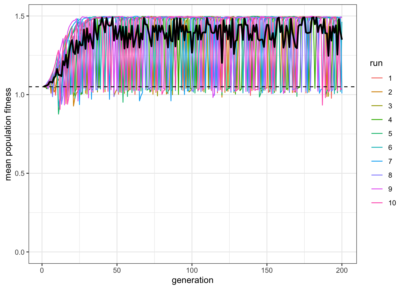
Figure 9.2: The average fitness of critical learners (black line) clearly exceeds the average fitness of populations entirely comprised of individual learners.
Yes: Even if there is still some noise, critical learners clearly outperform the dotted line indicating a hypothetical 100% individual learning population. Rogers’ paradox is solved.
9.2 Summary of the model
Several ‘solutions’ have been demonstrated to Rogers’ paradox. Here we have explored one of them. Critical learners can flexibly employ both social and individual learning, and do this in an adaptive manner (i.e. only individually learn if social learning is unsuccessful). Critical learners outperform the pure individual learning and pure social learning strategies. They, therefore, solve Rogers’ paradox by exceeding the mean fitness of a population entirely composed of individual learning.
One might complain that all this is obvious. Of course, real organisms can learn both socially and individually and adaptively employ both during their lifetimes. But hindsight is a wonderful thing. Before Rogers’ model, scholars did not fully recognise this, and simply argued that social learning is adaptive because it has lower costs than individual learning. We now know this argument is faulty. But it took a simple model to realise it and to realise the reasons why.
9.3 Further reading
There are several other solutions to Rogers’ paradox in the literature. Boyd and Richerson (1995) suggested individuals who initially learn individually and then if unsatisfied learn socially - the reverse of Enquist, Eriksson, and Ghirlanda (2007)‘s critical learners. Boyd and Richerson (1995) also suggested that if culture is cumulative, i.e. each generation builds on the beneficial modifications of the previous generations, then Rogers’ paradox is resolved.