Chapter 2 Unbiased and biased mutation
Evolution doesn’t work without a source of variation that introduces new variation upon which selection, drift and other processes can act. In genetic evolution, mutation is almost always blind with respect to function. Beneficial genetic mutations are no more likely to arise when they are needed than when they are not needed - in fact, most genetic mutations are neutral or detrimental to an organism. Cultural evolution is more interesting, in that novel variation may sometimes be directed to solve specific problems, or systematically biased due to features of our cognition. In the models below, we’ll simulate both unbiased and biased mutation.
2.1 Unbiased mutation
First, we will simulate unbiased mutation in the same basic model as used in the previous chapter. We’ll remove unbiased transmission to see the effect of unbiased mutation alone.
As in the previous model, we assume \(N\) individuals each of whom possesses one of two discrete cultural traits, denoted \(A\) and \(B\). In each generation, from \(t=1\) to \(t=t_{\text{max}}\), the \(N\) individuals are replaced with \(N\) new individuals. Instead of random copying, each individual now gives rise to a new individual with the same cultural trait as them. (Another way of looking at this is in terms of timesteps, such as years: the same \(N\) individual live for \(t_{\text{max}}\) years and keep their cultural trait from one year to the next.)
At each generation, however, there is a probability \(\mu\) that each individual mutates from their current trait to the other trait (the Greek letter Mu is the standard notation for the mutation rate in genetic evolution, and it has an analogous function here). For example, vegetarian individuals can decide to eat animal products, and vice versa. Remember, this is not copied from other individuals, as in the previous model, but can be thought of as an individual decision. Another way to see this is that the probability of changing trait applies to each individual independently; whether an individual mutates has no bearing on whether or how many other individuals have mutated. On average, this means that \(\mu N\) individuals mutate each generation. Like in the previous model, we are interested in tracking the proportion \(p\) of agents with trait \(A\) over time.
We’ll wrap this in a function called unbiased_mutation(), using much of the same code as unbiased_transmission_3(). As before, we need to call the tidyverse library in order to use the tibble command, and later commands like ggplot2.
library(tidyverse)

unbiased_mutation <- function(N, mu, p_0, t_max, r_max) {
  # Create the output tibble
  output <- tibble(generation = rep(1:t_max, r_max),
                   p = as.numeric(rep(NA, t_max * r_max)),
                   run = as.factor(rep(1:r_max, each = t_max)))

  for (r in 1:r_max) {
    population <- tibble(trait = sample(c("A", "B"), N, replace = TRUE,
                                        prob = c(p_0, 1 - p_0)))
    # Add first generation's p for run r
    output[output$generation == 1 & output$run == r, ]$p <-
      sum(population$trait == "A") / N
    for (t in 2:t_max) {
      # Copy individuals to previous_population tibble
      previous_population <- population

      # Determine 'mutant' individuals
      mutate <- sample(c(TRUE, FALSE), N, prob = c(mu, 1 - mu), replace = TRUE)

      # If there are 'mutants' from A to B
      if (nrow(population[mutate & previous_population$trait == "A", ]) > 0) {
        # Then flip them to B
        population[mutate & previous_population$trait == "A", ]$trait <- "B"
      }

      # If there are 'mutants' from B to A
      if (nrow(population[mutate & previous_population$trait == "B", ]) > 0) {
        # Then flip them to A
        population[mutate & previous_population$trait == "B", ]$trait <- "A"
      }

      # Get p and put it into output slot for this generation t and run r
      output[output$generation == t & output$run == r, ]$p <-
        sum(population$trait == "A") / N
    }
  }
  # Export data from function
  output
}
The only changes from the previous model are the addition of mu, the parameter that specifies the probability of mutation, in the function definition and new lines of code within the for loop on t which replace the random copying command with unbiased mutation. Let’s examine these lines to see how they work.
The most obvious way of implementing unbiased mutation - which is not done above - would have been to set up another for loop. We would cycle through every individual one by one, each time calculating whether it should mutate or not based on mu. This would certainly work, but R is notoriously slow at loops. It’s always preferable in R, where possible, to use ‘vectorised’ code. That’s what is done above in our three added lines, starting from mutate <- sample().
First, we pre-specify the probability of mutating for each individual. For this, we again use the function sample(), picking TRUE (corresponding to being a mutant) or FALSE (not mutating, i.e. keeping the same cultural trait) for \(N\) times. The draw, however, is not random: the probability of drawing TRUE is equal to \(\mu\), and the probability of drawing FALSE is \(1-\mu\). You can think about the procedure in this way: each individual in the population flips a biased coin that has \(\mu\) probability to land on, say, heads, and \(1-\mu\) to land on tails. If it lands on heads they change their cultural trait.
In the subsequent lines we change the traits for the ‘mutant’ individuals. We need to check whether there are individuals that change their trait, both from \(A\) to \(B\) and vice versa, using the two if conditionals. If there are no such individuals, then assigning a new value to an empty tibble returns an error. To avoid this, we make sure that the number of rows is greater than 0 (using nrow()>0 within the if).
To plot the results, we can use the same function plot_multiple_runs() we wrote in the previous chapter.
Let’s now run and plot the model:
data_model <- unbiased_mutation(N = 100, mu = 0.05, p_0 = 0.5, t_max = 200, r_max = 5)
plot_multiple_runs(data_model)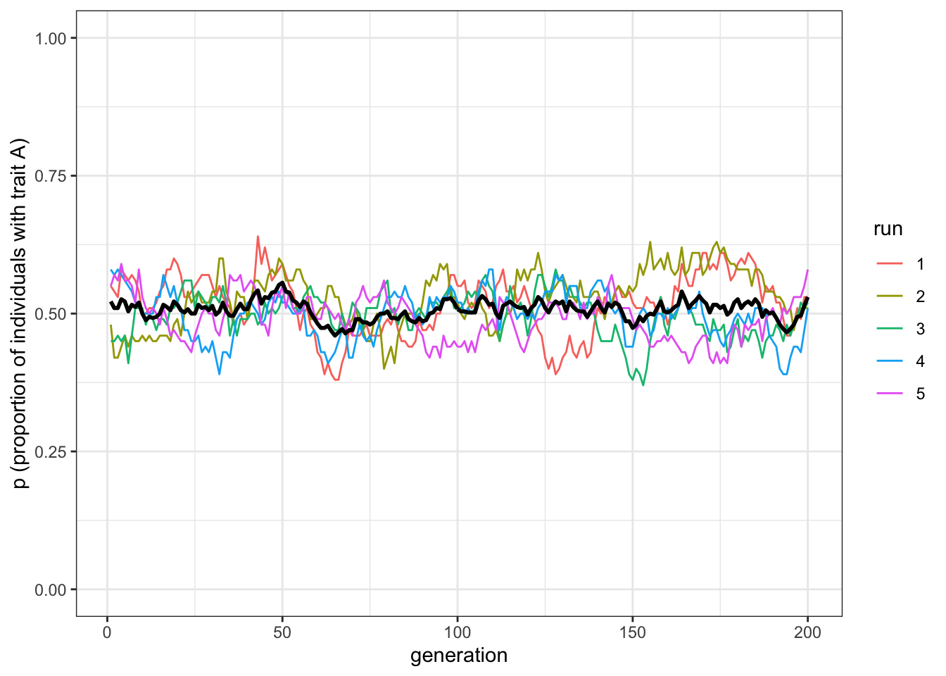
Figure 2.1: Trait frequencies fluctuate around 0.5 under unbiased mutation
Unbiased mutation produces random fluctuations over time and does not alter the overall frequency of \(A\), which stays around \(p=0.5\). Because mutations from \(A\) to \(B\) are as equally likely as \(B\) to \(A\), there is no overall directional trend.
If you remember from the previous chapter, with unbiased transmission, when populations were small (e.g. \(N=100\)) generally one of the traits disappeared after a few generations. Here, though, with \(N=100\), both traits remain until the end of the simulation. Why this difference? You can think of it in this way: when one trait becomes popular, say the frequency of \(A\) is equal to \(0.8\), with unbiased transmission it is more likely that individuals of the new generation will pick up \(A\) randomly when copying. The few individuals with trait \(B\) will have 80% probability of copying \(A\). With unbiased mutation, on the other hand, since \(\mu\) is applied independently to each individual, when \(A\) is common then there will be more individuals that will flip to \(B\) (specifically, \(\mu p N\) individuals, which in our case is 4) than individuals that will flip to \(A\) (equal to \(\mu (1-p) N\) individuals, in our case 1) keeping the traits at similar frequencies.
But what if we were to start at different initial frequencies of \(A\) and \(B\)? Say, \(p=0.1\) and \(p=0.9\)? Would \(A\) disappear? Would unbiased mutation keep \(p\) at these initial values, like we saw unbiased transmission does in Model 1?
To find out, let’s change \(p_0\), which specifies the initial probability of drawing an \(A\) rather than a \(B\) in the first generation.
data_model <- unbiased_mutation(N = 100, mu = 0.05, p_0 = 0.1, t_max = 200, r_max = 5)
plot_multiple_runs(data_model)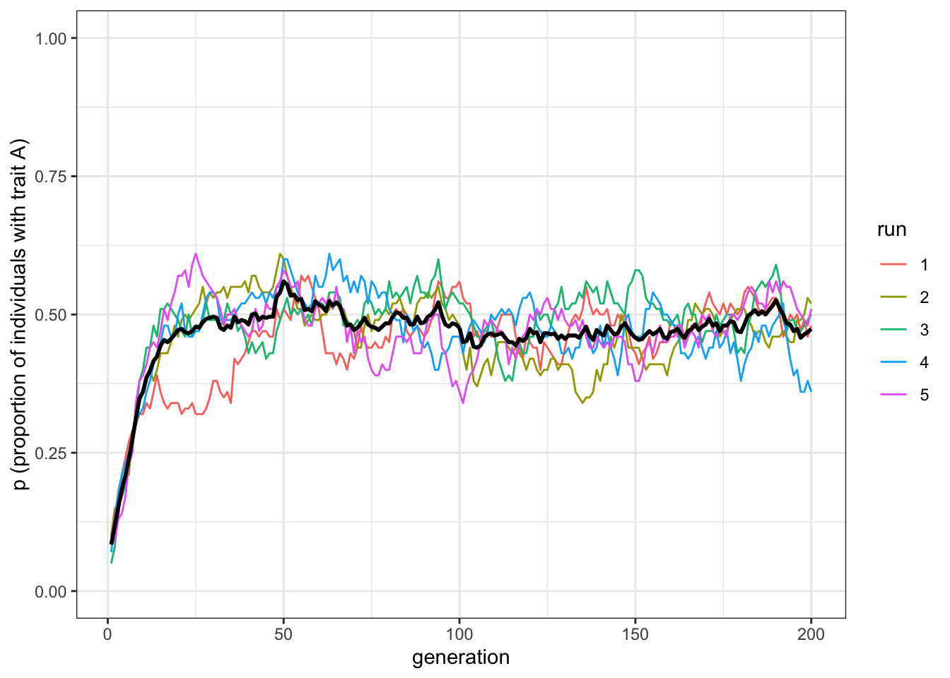
Figure 2.2: Unbiased mutation causes trait frequencies to converge on 0.5, irrespective of starting frequencies
You should see \(p\) go from \(0.1\) up to \(0.5\). In fact, whatever the initial starting frequencies of \(A\) and \(B\), unbiased mutation always leads to \(p=0.5\), for the reason explained above: unbiased mutation always tends to balance the proportion of \(A\)s and \(B\)s.
2.2 Biased mutation
A more interesting case is biased mutation. Let’s assume now that there is a probability \(\mu_b\) that an individual with trait \(B\) mutates into \(A\), but there is no possibility of trait \(A\) mutating into trait \(B\). Perhaps trait \(A\) is a particularly catchy or memorable version of a story or an intuitive explanation of a phenomenon, and \(B\) is difficult to remember or unintuitive to understand.
The function biased_mutation() captures this unidirectional mutation.
biased_mutation <- function(N, mu_b, p_0, t_max, r_max) {
   # Create the output tibble
  output <- tibble(generation = rep(1:t_max, r_max),
                   p = as.numeric(rep(NA, t_max * r_max)),
                   run = as.factor(rep(1:r_max, each = t_max)))

  for (r in 1:r_max) {
    population <- tibble(trait = sample(c("A", "B"), N, replace = TRUE,
                                        prob = c(p_0, 1 - p_0)))
    # Add first generation's p for run r
    output[output$generation == 1 & output$run == r, ]$p <-
      sum(population$trait == "A") / N
    for (t in 2:t_max) {
      # Copy individuals to previous_population tibble
      previous_population <- population

      # Determine 'mutant' individuals
      mutate <- sample(c(TRUE, FALSE), N, prob = c(mu_b, 1 - mu_b), replace = TRUE)

      # If there are 'mutants' from B to A
      if (nrow(population[mutate & previous_population$trait == "B", ]) > 0) {
        # Then flip them to A
        population[mutate & previous_population$trait == "B", ]$trait <- "A"
      }
      # Get p and put it into output slot for this generation t and run r
      output[output$generation == t & output$run == r, ]$p <-
        sum(population$trait == "A") / N
    }
  }
  # Export data from function
  output
}
There are just two changes in this code compared to unbiased_mutation(). First, we’ve replaced mu with mu_b to keep the two parameters distinct and avoid confusion. Second, the line in unbiased_mutation() which caused individuals with \(A\) to mutate to \(B\) has been deleted.
Let’s see what effect this has by running biased_mutation(). We’ll start with the population entirely composed of individuals with \(B\), i.e. \(p_0=0\), to see how quickly and in what manner \(A\) spreads via biased mutation.
data_model <- biased_mutation(N = 100, mu_b = 0.05, p_0 = 0, t_max = 200, r_max = 5)
plot_multiple_runs(data_model)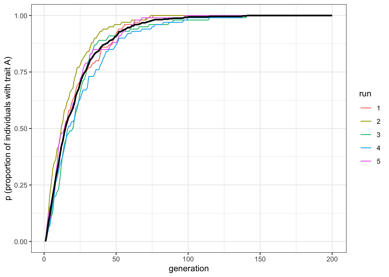
Figure 2.3: Biased mutation causes the favoured trait to replace the unfavoured trait
The plot shows a steep increase that slows and plateaus at \(p=1\) by around generation \(t=100\). There should be a bit of fluctuation in the different runs, but not much. Now let’s try a larger sample size.
data_model <- biased_mutation(N = 10000, mu_b = 0.05, p_0 = 0, t_max = 200, r_max = 5)
plot_multiple_runs(data_model)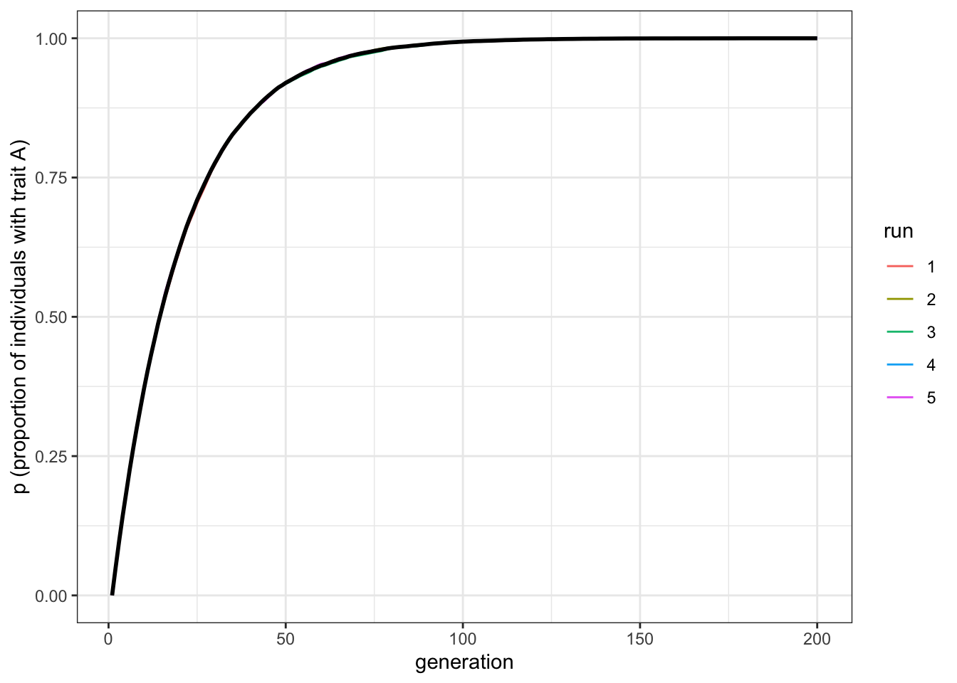
Figure 2.4: Increasing the population size does not change the rate at which biased mutation causes the favoured trait to increase in frequency
With \(N = 10000\) the line should be smooth with little (if any) fluctuation across the runs. But notice that it plateaus at about the same generation, around \(t=100\). Population size has little effect on the rate at which a novel trait spreads via biased mutation. \(\mu_b\), on the other hand, does affect this speed. Let’s double the biased mutation rate to 0.1.
data_model <- biased_mutation(N = 10000, mu_b = 0.1, p_0 = 0, t_max = 200, r_max = 5)
plot_multiple_runs(data_model)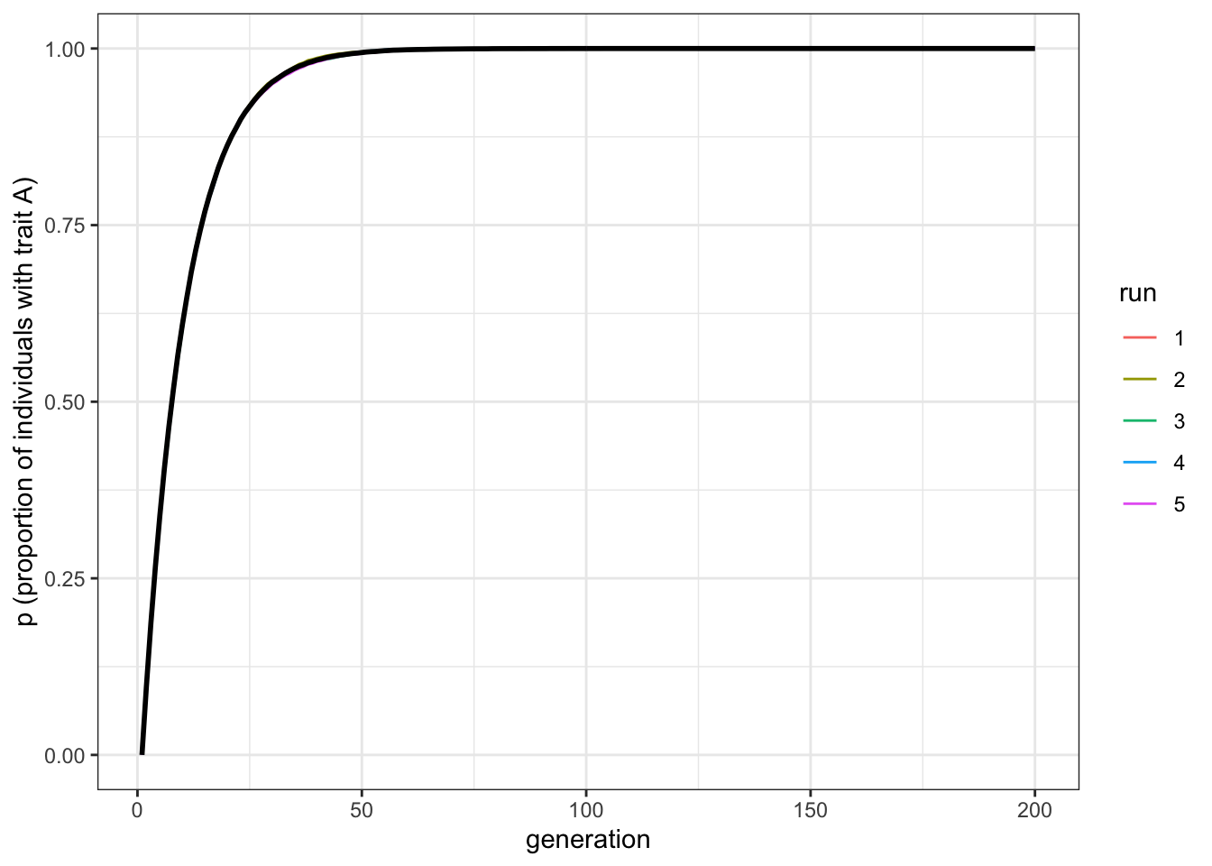
Figure 2.5: Increasing the mutation rate increases the rate at which biased mutation causes the favoured trait to increase in frequency
Now trait \(A\) reaches fixation around generation \(t=50\). Play around with \(N\) and \(\mu_b\) to confirm that the latter determines the rate of diffusion of trait \(A\), and that it takes the same form each time - roughly an ‘r’ shape with an initial steep increase followed by a plateauing at \(p=1\).
2.3 Summary of the model
With this simple model, we can draw the following insights. Unbiased mutation, which resembles genetic mutation in being non-directional, always leads to an equal mix of the two traits. It introduces and maintains cultural variation in the population. It is interesting to compare unbiased mutation to unbiased transmission from the previous chapter. While unbiased transmission did not change \(p\) over time, unbiased mutation always converges on \(p=0.5\), irrespective of the starting frequency. (NB \(p = 0.5\) assuming there are two traits; more generally, \(p=1/v\), where \(v\) is the number of traits.)
Biased mutation, which is far more common - perhaps even typical - in cultural evolution, shows different dynamics. Novel traits favoured by biased mutation spread in a characteristic fashion - an r-shaped diffusion curve - with a speed characterised by the mutation rate \(\mu_b\). Population size has little effect, whether \(N = 100\) or \(N = 10000\). Whenever biased mutation is present (\(\mu_b>0\)), the favoured trait goes to fixation, even if it is not initially present.
In terms of programming techniques, the major novelty in this model is the use of sample() to determine which individuals should undergo whatever the fixed probability specifies (in our case, mutation). This could be done with a loop, but vectorising code in the way we did here is much faster in R than loops.
2.4 Further reading
Boyd and Richerson (1985) model what they call ‘guided variation,’ which is equivalent to biased mutation as modelled in this chapter. Henrich (2001) shows how biased mutation / guided variation generates r-shaped curves similar to those generated here.