Chapter 15 Group structured populations and migration

For mathematical and computational simplicity, we often assume that populations are well-mixed. That is, individuals have an equal chance of encountering or interacting with any other individual. In the previous chapter we have looked at the effects of structured interactions on the transmission of cultural traits. Both structured and unstructured interactions can be good approximations of the real world, depending on the context and research question. What about structured populations, a combination of the two? That is, a large population of individuals is divided into subsets, where individuals are more likely to encounter those from the same subset but much less likely to encounter others from a different one. Here, learning would almost exclusively occur within each subset. However, individuals may migrate between subsets, bringing along their own repertoire of cultural traits, or might visit another subset and then return with new cultural variants. In this chapter, we will take a closer look at these two scenarios.

15.1 Modelling migration and contact between population subsets

Before we model subset populations, let us begin by developing a simple transmission model, similar to what we have done in the first chapter of this book. We start with a population of size $n$, and $b$ instances of a behavioural trait. That is, an individual will only ever have one version of a behaviour, for example, greeting another individual with a handshake or by bumping elbows. We choose this to keep the example simple. Other possibilities would be, for example, to model the migration of distinct behaviours.

Let us set up a population. Because we are only interested in which instance of a particular behaviour an individual expresses, each individual can be fully described by that instance, and so, we can represent the entire population as a vector of expressed behaviours (behaviours).

n <- 100
b <- 2

behaviours <- sample(x = b, size = n, replace = TRUE)
table(behaviours)

## behaviours
##  1  2 
## 51 49

The table() function counts each element of a given vector. It is similar to tabulate() which we used previously, however, table() returns a named vector, so that you know exactly which element is present how many times.

Each individual in our population expresses only one behaviour. Occasionally, one of the individuals will copy the behaviour of another individual. To simulate this, we select a random individual, which copies a randomly selected behaviour from the population. This approach is identical to the unbiased learning in our earlier chapters. We can simulate repeated updating events by wrapping a for loop around the code. Additionally, we will add a record variable (rec_behav) to store the frequency of each behaviour.

library(tidyverse)
r_max <- 1000
rec_behav <- tibble(time = 1:r_max, b1 = 0, b2 = 0)

for(round in 1:r_max){
  # Unbiased copying of a behaviour by a random individual
  behaviours[ sample(x = n, size = 1) ] <- sample(x = behaviours, size = 1)
  # Record the frequency of each trait in each round
  rec_behav[round, "b1"] <- sum(behaviours==1)
  rec_behav[round, "b2"] <- sum(behaviours==2)
}
rec_behav

## # A tibble: 1,000 x 3
##     time    b1    b2
##    <int> <dbl> <dbl>
##  1     1    50    50
##  2     2    49    51
##  3     3    50    50
##  4     4    50    50
##  5     5    50    50
##  6     6    50    50
##  7     7    50    50
##  8     8    50    50
##  9     9    50    50
## 10    10    50    50
## # … with 990 more rows

To plot the results with ggplot(), we need to turn the ‘wide’ data (where repeated measures/different categories are in the same line) into ‘long’ data (where each line has only one observation/category). To ‘rotate’ our data we can use the pivot_longer() function. In its arguments we tell it to combine the results of columns b1 and b2 into beaviour, which indicates the name of the behaviour, and freq, which is the frequency of that behaviour. The function will repeat the entries of the time column accordingly:

rec_behav_l <- pivot_longer(data = rec_behav, names_to = "behaviour", 
                            values_to = "freq", cols=c("b1","b2"))
rec_behav

## # A tibble: 1,000 x 3
##     time    b1    b2
##    <int> <dbl> <dbl>
##  1     1    50    50
##  2     2    49    51
##  3     3    50    50
##  4     4    50    50
##  5     5    50    50
##  6     6    50    50
##  7     7    50    50
##  8     8    50    50
##  9     9    50    50
## 10    10    50    50
## # … with 990 more rows

rec_behav_l

## # A tibble: 2,000 x 3
##     time behaviour  freq
##    <int> <chr>     <dbl>
##  1     1 b1           50
##  2     1 b2           50
##  3     2 b1           49
##  4     2 b2           51
##  5     3 b1           50
##  6     3 b2           50
##  7     4 b1           50
##  8     4 b2           50
##  9     5 b1           50
## 10     5 b2           50
## # … with 1,990 more rows

Now, we can plot the frequency of each behaviour over time:

ggplot(rec_behav_l) + 
  geom_line(aes(x = time, y = freq/n, col = behaviour)) + 
  scale_y_continuous(limits = c(0,1)) + 
  ylab("proportion of population with behaviour") +
  theme_bw()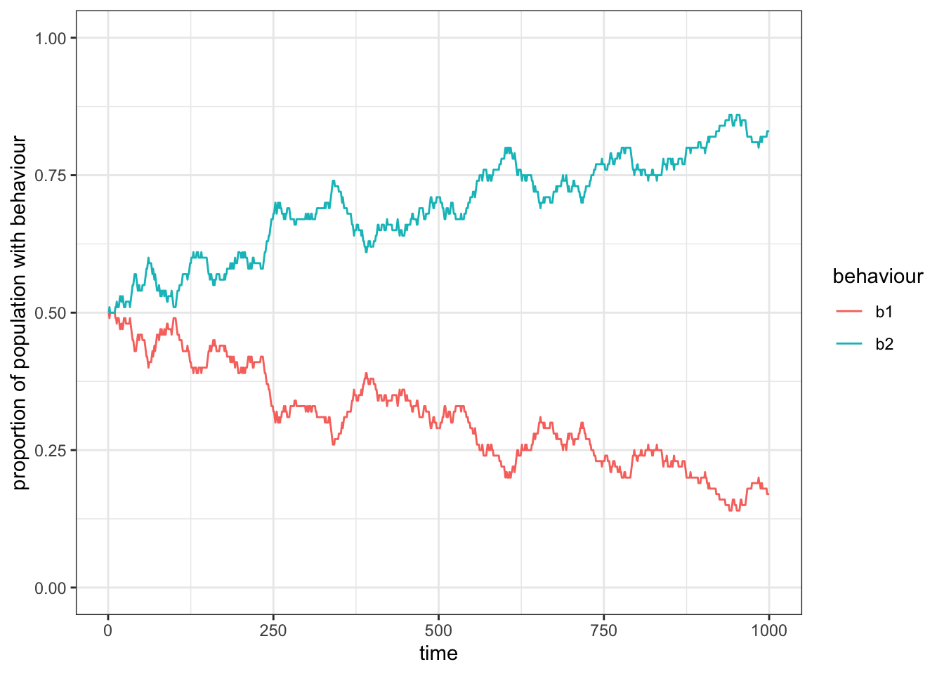

Figure 15.1: On average the frequenca of two behaviours that are transmitted without a bias will fluctuate around 0.5.

As we would expect from an unbiased transmission, the frequency of the two traits will move around $0.5$.

We can wrap this code in a function to make it easier to use in the future:

structured_population_1 <- function(n, b, r_max){
  behaviours <- sample(x = 1:b, size = n, replace = TRUE)
  rec_behav <- matrix(NA, nrow = r_max, ncol = b)
  
  for(round in 1:r_max){
    # Unbiased copying of a behaviour by a random individual
    behaviours[ sample(x = n, size = 1) ] <- sample(x = behaviours, size = 1)
    rec_behav[round,] <- unlist(lapply(1:b, function(B) sum(behaviours==B))) / n
  }
  # Turn matrix into tibble
  rec_behav_tbl <- as_tibble(rec_behav)
  # Set column names to b1, b2 to represent the behaviours
  colnames(rec_behav_tbl) <- paste("b" ,1:b, sep = "")
  # Add a column for each round
  rec_behav_tbl$time <- 1:r_max
  # Turn wide format into long format data
  rec_behav_tbl_l <- pivot_longer(data = rec_behav_tbl, names_to = "behaviour", values_to = "freq", !time)
  # Return result
  return(rec_behav_tbl_l)
}

Note that we initially create the matrix rec_behav, which we then convert to a tibble object. The advantage here is that we can quickly create a matrix of a certain size (here, the number of rounds times number of behaviours), in which we can record the frequencies of each behaviour. The tibble, however, will make handling and plotting our data easier.

Let us test what would happen if we ran this simulation with a very small population size of $n=20$:

# Run simulation
res <- structured_population_1(n = 20, b = 2, r_max = 1000)

# Plot results
ggplot(res) + 
  geom_line(aes(x = time, y = freq, col = behaviour)) + 
  scale_y_continuous(limits = c(0,1)) + 
  ylab("proportion of population with behaviour") +
  theme_bw()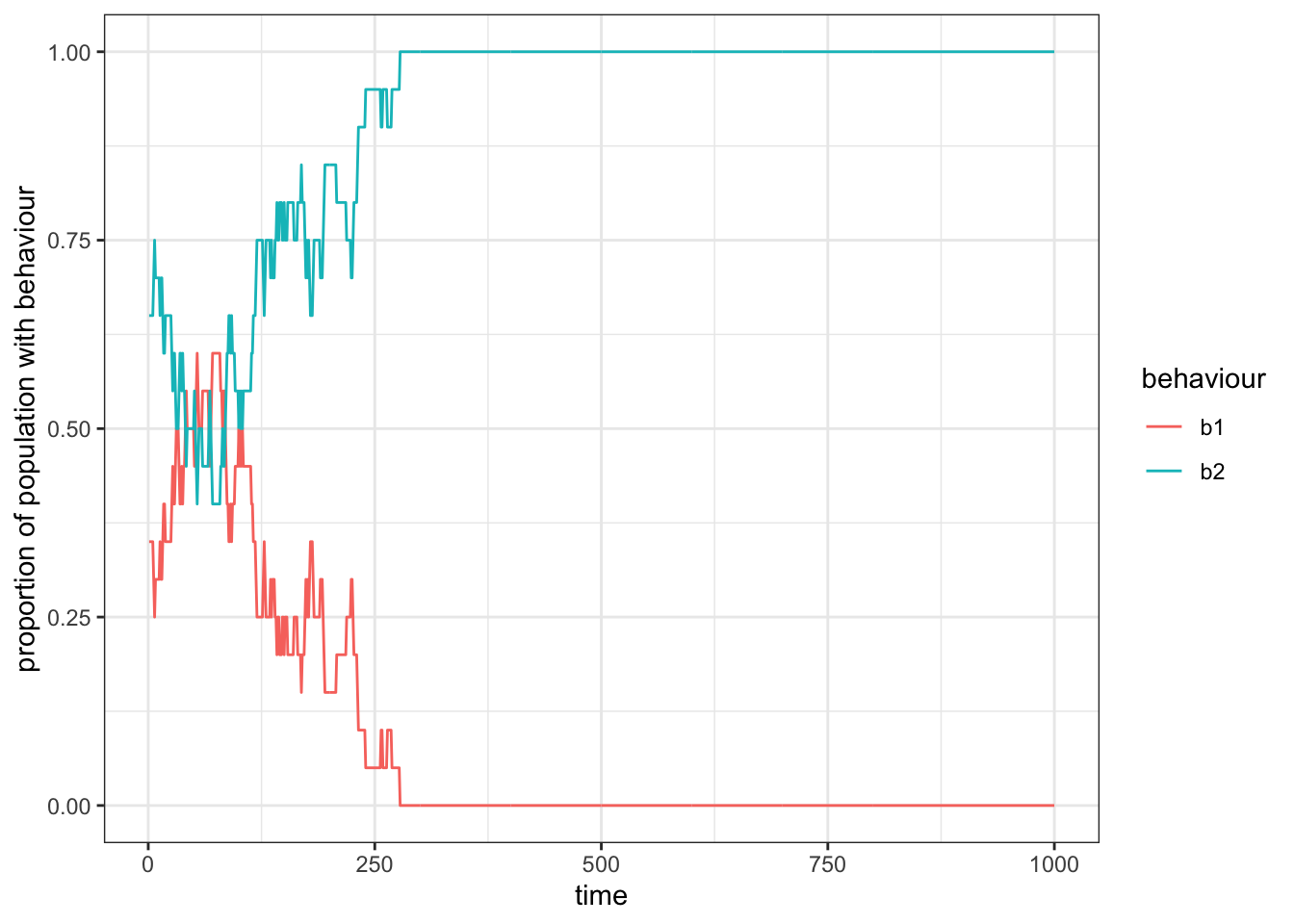

In smaller populations (here, $n=20$), drift will lead to the exclusion of one of the two behaviours from the group, such that the other behaviour becomes fixed.

Figure 15.2: In smaller populations (here, $n=20$), drift will lead to the exclusion of one of the two behaviours from the group, such that the other behaviour becomes fixed.

We observe that the two behaviours fluctuate around $0.5$ until, by chance, one behaviour is completely replaced by the other one. This is simply due to drift, which affects all small populations or very long time scales, as we already saw in the first chapter.

15.2 Subdivided population with limited contact

Let us now move on from the single population to a population that is divided into subsets (we will call them clusters, as subset() is already taken by a generic function in R). For simplicity, we will assume only two instances of a behaviour. That way, we only need to track the frequency of one behaviour, $p$, in each subset. We will also assume that there are the same number, $n$, of individuals in each cluster, $c$.

structured_population_2 <- function(n, c, r_max){
  total_pop <- c * n
  cluster <- rep(1:c, each = n)
  behaviours <- sample(x = 2, size = total_pop, replace = TRUE)
  rec_behav <- matrix(NA, nrow = r_max, ncol = c)
  
  for(round in 1:r_max){
    behaviours[ sample(x = total_pop, size = 1) ] <- sample(x = behaviours, size = 1)
    # Recalculate p for each cluster
    for(clu in 1:c){
      rec_behav[round, clu] <- sum(behaviours[cluster == clu] == 1) / n
    }
  }
  rec_behav_tbl <- as_tibble(rec_behav)
  # Set column names to c1, c2 to represent each cluster
  colnames(rec_behav_tbl) <- paste("c", 1:c, sep = "")
  rec_behav_tbl$time <- 1:r_max
  rec_behav_tbl_l <- pivot_longer(data = rec_behav_tbl, names_to = "cluster", 
                                  values_to = "p", !time)
  return(rec_behav_tbl_l)
}

This function is very similar to migration_model_1() but accounts for the additional clusters. For example, the columns of rec_behav now store $p$ for each cluster. We calculate these values in every time step. We could also just calculate it for the cluster of the observing individual, however, if we keep the calculation more general, we will not have to change the code should we want individuals to be able to permanently move from one cluster to another. In that case we would need to calculate $p$ for both clusters.

Also, note that this time we did not tell pivot_longer() which columns to pivot but which one we want to keep unchanged (!time). This is because we do not know the numbers of columns before we run the simulation. Therefore, it is easier to just make an exception for the time column.

Let us run the simulation for 4 subsets with each 50 individuals:

res <- structured_population_2(n = 50, c = 4, r_max = 1000)

ggplot(res) + 
  geom_line(aes(x = time, y = p, col = cluster)) + 
  scale_y_continuous(limits = c(0,1)) + 
  ylab("proportion of behaviour 1 in cluster") + 
  theme_bw()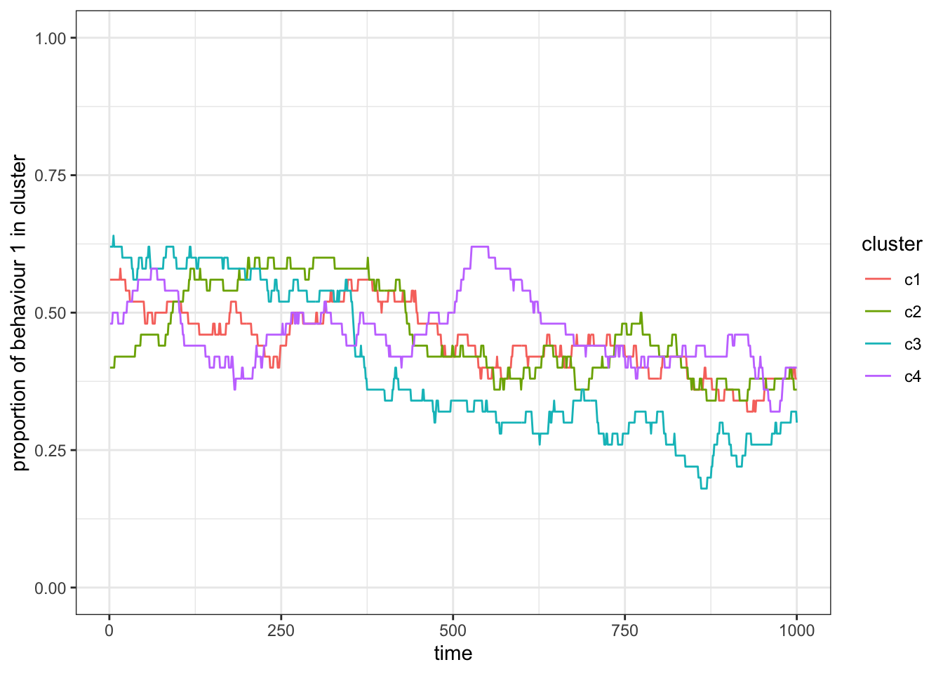

The frequency of one out of two behaviours in two subsets will fluctuate around 0.5 if individuals are equally likely to learn from individuals in both subsets (or clusters).

Figure 15.3: The frequency of one out of two behaviours in two subsets will fluctuate around 0.5 if individuals are equally likely to learn from individuals in both subsets (or clusters).

You will observe two things. First, on average the frequency of each behaviour will still be around $0.5$, and second that the frequency changes are correlated between all subsets. This is expected because, with the current version of our model, individuals do not distinguish between or have different access to individuals of either cluster. In fact, the fluctuations we observe here are purely stochastic and based on the relatively small subsets (try running the code with e.g. $N=1000$).

Let us now move on to the case where members of a subset preferentially learn from others within their cluster. This might be the case where individuals spent most of their time in their subsets and only occasionally interact with individuals from other subsets. To simulate this, we can use most of the code from structured_population_2() with a few small changes. First, we will change the sample() function. Instead of sampling demonstrators across the entire population, we want the observer to preferentially (or exclusively) choose someone from its own cluster. To achieve this, we will use the prob. This argument defines a weight (or probability) with which an element of a provided set is chosen. By default, each element has a weight of $1$ (or a probability of $1/N$) and thus is equally likely to be selected. To limit our scope to individuals within the same cluster, we can simply set the weight to $0$ for all individuals that are in a different cluster and to $1$ for those that are in the same cluster. Assuming an individual is in cluster 2 then we select all other individuals in the same cluster using cluster == cluster_id, where cluster_id is 2. This will return a vector with TRUE and FALSE values. We can turn this into weights (i.e. 0s and 1s) simply by multiplying the vector with 1, R will then automatically turn the logical into a numeric vector. Additionally, we will select two individuals from the cluster, an observer, and a demonstrator (or model). Of course, we can only perform this, if there are at least 2 individuals in the cluster. Take a look at the new function:

structured_population_3 <- function(n, c, r_max){
  total_pop <- c * n
  cluster <- rep(1:c, each = n)
  behaviours <- sample(x = 2, size = total_pop, replace = TRUE)
  rec_behav <- matrix(NA, nrow = r_max, ncol = c)
  
  for(round in 1:r_max){
    # Choose a random cluster
    cluster_id <- sample(c, 1)
    # If there are at least two individuals in this cluster
    if(sum(cluster == cluster_id)>1){
      # Choose a random observer and a random individual to observe within the same cluster 
      observer_model <- sample(x = total_pop, size = 2, replace = F, 
                               prob = (cluster == cluster_id)*1)
      behaviours[ observer_model[1] ] <- behaviours[ observer_model[2] ]
    }

    for(clu in 1:c){
      rec_behav[round, clu] <- sum(behaviours[cluster == clu] == 1) / n
    }
  }
  return(matrix_to_tibble(m = rec_behav))
}

You might have noticed a new function at the very end: matrix_to_tibble(). This is a little helper function. As we keep turning matrices into tibbles, changing their column names, and adding a time column at the end of our simulation, we can also separate this process in its own function to reuse it in the future versions of our simulation function. This is generally useful whenever you have a piece of code that you keep replicating. This is what the helper function looks like:

matrix_to_tibble <- function(m){
  m_tbl <- as_tibble(m)
  colnames(m_tbl) <- paste("c" ,1:ncol(m), sep = "")
  m_tbl$time<- 1:nrow(m)
  m_tbl_l <- pivot_longer(data = m_tbl, names_to = "cluster", values_to = "p", !time)
  return(m_tbl_l)
}

Let us run a simple example with three subsets and each $n=20$:

res <- structured_population_3(n = 20, c = 3, r_max = 1000)
ggplot(res) + 
  geom_line(aes(x = time, y = p, col = cluster)) + 
  scale_y_continuous(limits = c(0,1)) + 
  ylab("proportion of behaviour 1 in cluster") + 
  theme_bw()

When individuals copy behaviours only from individuals within their own subset, we find that the frequency of behaviour 1 becomes uncorrelated between the two subsets. In this example, behaviour 1 is lost in cluster 2, whereas it is still present in cluster 1 at the end of the simulation.

Figure 15.4: When individuals copy behaviours only from individuals within their own subset, we find that the frequency of behaviour 1 becomes uncorrelated between the two subsets. In this example, behaviour 1 is lost in cluster 2, whereas it is still present in cluster 1 at the end of the simulation.

When we run this simulation repeatedly, you will see that sometimes behaviour 1 gets lost in one, both, or neither of the clusters. Because in this iteration of our simulation there are no interactions between individuals of different clusters, we are essentially simulating three (small) independent populations.

Let us change the code so that we can alter the rate at which individuals from different subsets might encounter each other. In mathematical terms, let $\omega = s$ be the probability to observe another individual, with $s = 0$ for individuals of another subset and $s=1$ for individuals of the same subset. We can alter $\omega$ to allow interaction with individuals from another subset by adding a contact probability, $p_c$, such that $\omega = \frac{s + p_c}{1+p_c}$. We divide by $1+p_c$ so that $0 \leq \omega \leq 1$. With this change the probability to encounter an individual from any subset is at least $p_c$. Take a look at the updated function:

structured_population_4 <- function(n, c, p_c, r_max){
  total_pop <- c * n
  cluster <- rep(1:c, each = n)
  behaviours <- sample(x = 2, size = total_pop, replace = TRUE)
  rec_behav <- matrix(NA, nrow = r_max, ncol = c)
  
  for(round in 1:r_max){
    cluster_id <- sample(c, 1)
    s <- cluster == cluster_id
    if(sum(s)>1){
      # Choose a random observer and a random individual to observe within the same cluster 
      observer_model <- sample(x = total_pop, size = 2, replace = F, 
                               prob = (s + p_c) / (1 + p_c))
      behaviours[ observer_model[1] ] <- behaviours[ observer_model[2] ]
    }
    
    for(clu in 1:c){
      rec_behav[round, clu] <- sum(behaviours[cluster == clu] == 1) / n
    }
  }
  return(matrix_to_tibble(m = rec_behav))
}

Let us now run simulations for different contact probabilities. We will simulate five subsets and use $p_c \in \{0, 0.1, 1 \}$, i.e. no contact, some contact, and full contact:

res_0  <- structured_population_4(n = 20, c = 5, p_c = 0, r_max = 1000)
res_01 <- structured_population_4(n = 20, c = 5, p_c = 0.1, r_max = 1000)
res_1  <- structured_population_4(n = 20, c = 5, p_c = 1, r_max = 1000)

ggplot(res_0) + 
  geom_line(aes(x = time, y = p, col = cluster)) + 
  scale_y_continuous(limits = c(0,1)) + 
  ylab("proportion of behaviour 1 in cluster") + 
  theme_bw()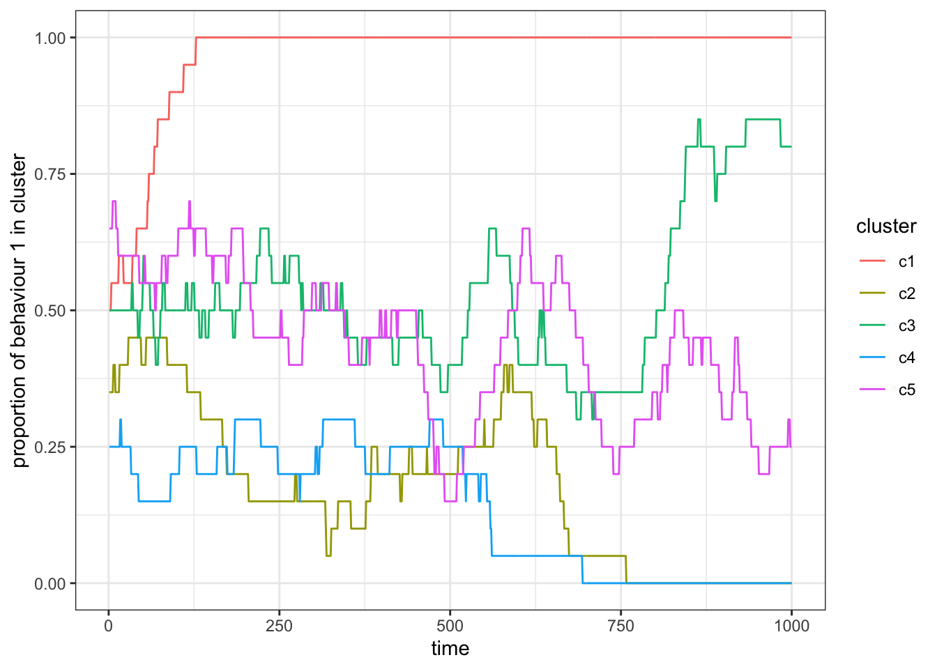

Figure 15.5: Simulation with no contact, $p_c = 0$.

ggplot(res_01) + 
  geom_line(aes(x = time, y = p, col = cluster)) + 
  scale_y_continuous(limits = c(0,1)) + 
  ylab("proportion of behaviour 1 in cluster") + 
  theme_bw()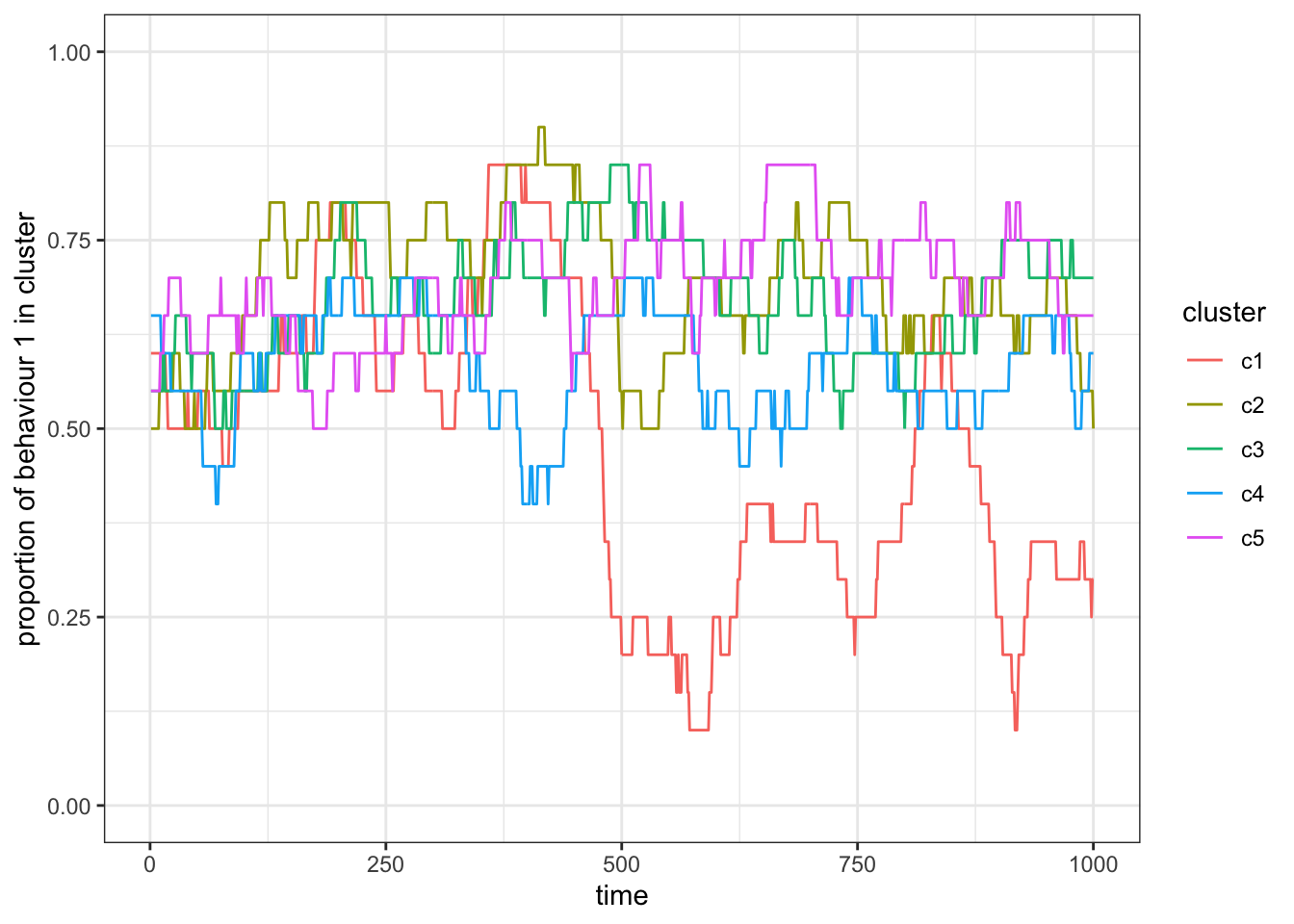

Figure 15.6: Simulation with some contact, $p_c = 0.1$.

ggplot(res_1) + 
  geom_line(aes(x = time, y = p, col = cluster)) + 
  scale_y_continuous(limits = c(0,1)) + 
  ylab("proportion of behaviour 1 in cluster") + 
  theme_bw()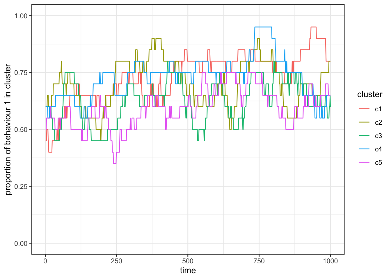

Figure 15.7: Simulation with full contact, $p_c = 1$.

With $p_c = 0$, the subsets (again) act as independent populations that fluctuate stochastically. As we increase $p_c$ the subsets become more correlated in the proportion of behaviour 1. For $p_c=1$ we recover a population without subsets.

15.3 Subdivided populations with migration

In the previous section we have modelled the movement of cultural traits between subsets due to occasional interactions. Let us now simulate the movement of individuals (and their cultural trait) between subsets. To model migration, we will add a migration probability $p_m$ to the model (with no migration where $p_m=0$, and always migrating to a random subset where $p_m=1$):

structured_population_5 <- function(n, c, p_c, p_m, r_max){
  total_pop <- c * n
  cluster <- rep(1:c, each = n)
  behaviours <- sample(x = 2, size = total_pop, replace = TRUE)
  rec_behav <- matrix(NA, nrow = r_max, ncol = c)
  
  for(round in 1:r_max){
    cluster_id <- sample(c, 1)
    s <- cluster == cluster_id
    if(sum(s)>1){
      observer_model <- sample(x = total_pop, size = 2, replace = F, 
                               prob = (s + p_c) / (1 + p_c))
      behaviours[ observer_model[1] ] <- behaviours[ observer_model[2] ]
    }
    
    # Migration to another cluster with probability p_m and if there is more than 
    # one subset
    if((runif(1,0,1) <= p_m) & (c > 1)){
      # Set cluster id that is different from the current one
      cluster[ observer_model[1] ] <- sample((1:c)[-cluster_id], 1)
    }
    
    for(clu in 1:c){
      rec_behav[round, clu] <- sum(behaviours[cluster == clu] == 1) / sum(cluster == clu)
    }
  }
  return(matrix_to_tibble(m = rec_behav))
}

The migration code chunk is doing two things. First, we make sure that migration only happens with the migration probability $p_m$ (for that, we compare a random value from a uniform distribution with p_m: runif(1,0,1) <= p_m) and only if the population is actually subset (c>1). And second, if the statement is TRUE, we choose one new cluster ID among all cluster IDs but without the current one (sample((1:c)[-cluster_id], 1)).

Let us run the simulation for three different migration probabilities, $p_m \in \{0, 0.1, 1 \}$. Let us also run the simulations much longer so that we will get to a case where a behaviour might get fixed in the subsets or the population:

res_0  <- structured_population_5(c = 5, n = 50, r_max = 10000, p_m = 0, p_c=0)
res_1  <- structured_population_5(c = 5, n = 50, r_max = 10000, p_m = 1, p_c=0)
res_01 <- structured_population_5(c = 5, n = 50, r_max = 10000, p_m = 0.1, p_c=0)

ggplot(res_0) + 
  geom_line(aes(x = time, y = p, col = cluster)) +
  scale_y_continuous(limits = c(0,1)) + 
  ylab("relative frequency of behaviour 1") + 
  theme_bw()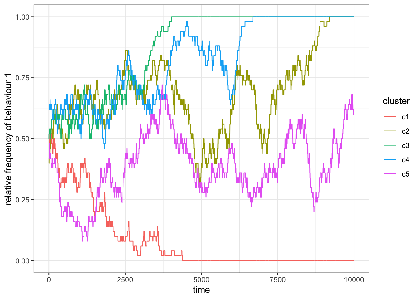

Figure 15.8: Without migration between clusters, there is no learning outside a subset, and so subsets act as independent populations.

For $p_m=0$ we find that the subsets act independently and fix either on behaviour 1 or 2.

ggplot(res_1) + 
  geom_line(aes(x = time, y = p, col = cluster)) +
  scale_y_continuous(limits = c(0,1)) + 
  ylab("relative frequency of behaviour 1") + 
  theme_bw()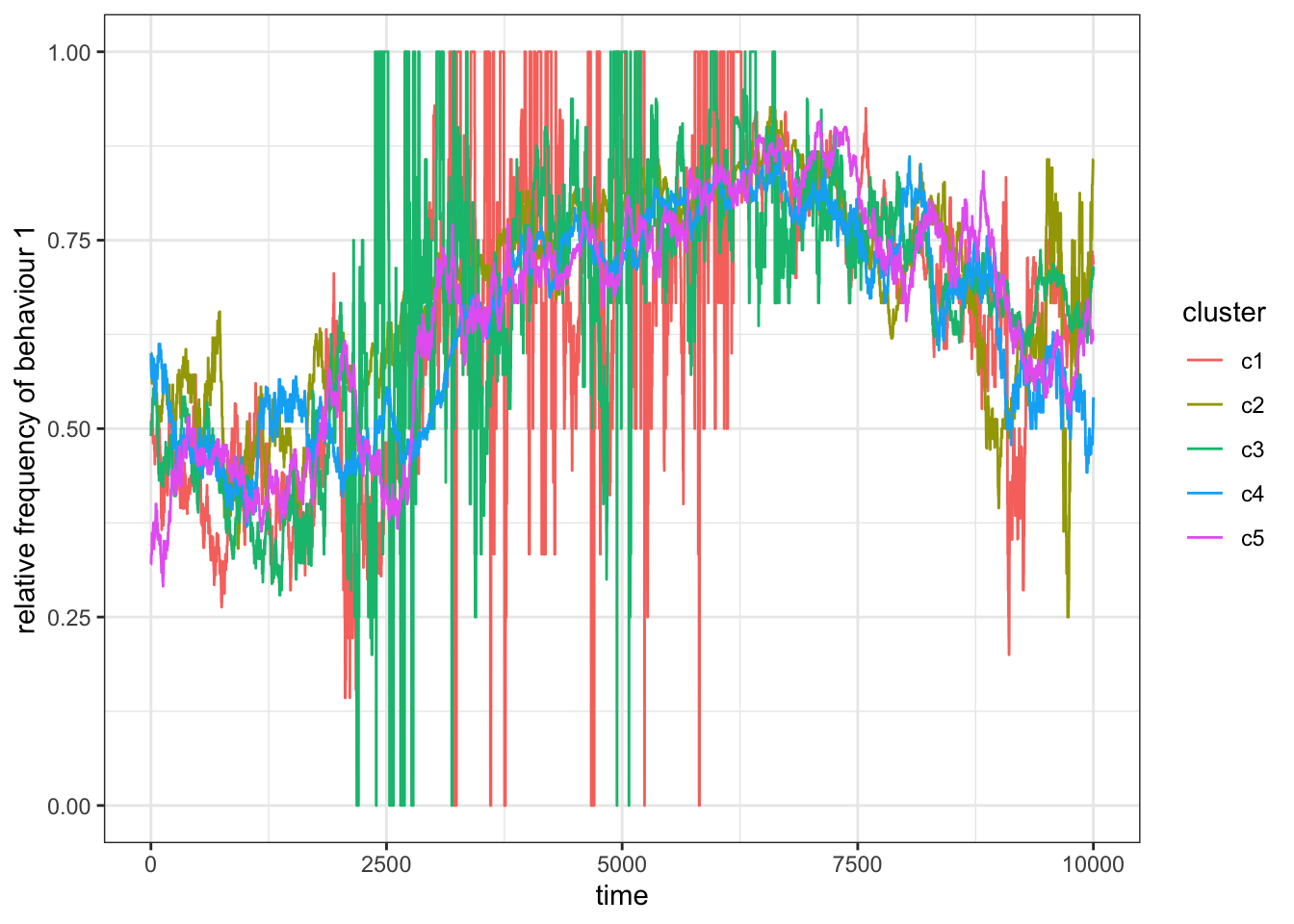

Figure 15.9: When $p_m=1$ the subsets act again as a single population.

For $p_m=1$, we find that the frequency of the behaviours become correlated as more and more individuals keep moving between the clusters. Eventually, all subsets will settle on the same behaviour. You might have also noticed that sometimes the curve for one or more subsets jumps between 0 and 1. This is the case when a subset is almost empty. Imagine a subset with only one individual with behaviour 1, then $p=1$. If this individual leaves the subset the curve jumps to $p=0$. We are less likely to observe empty subsets if we let them start out bigger (say $N=100$).

ggplot(res_01) + 
  geom_line(aes(x = time, y = p, col = cluster)) +
  scale_y_continuous(limits = c(0,1)) + 
  ylab("relative frequency of behaviour 1") + 
  theme_bw()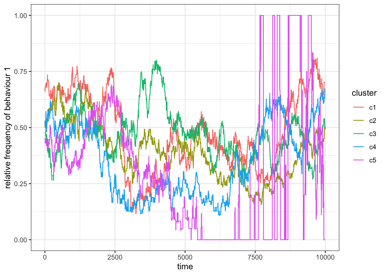

When migration is rare, the frequency of behaviour 1 changes occassionally but quickly bounes back to the original value in the subset.

Figure 15.10: When migration is rare, the frequency of behaviour 1 changes occassionally but quickly bounes back to the original value in the subset.

For rare migration ($p_m=0.1$), we sometimes find the population to fix on one behaviour, on two, or neither.

15.4 Varying contact and migration probability for repeated simulation runs

We have seen that both the migration and the contact probability affect the distribution of behaviour 1 and 2 in the population. In this last section let us run the model for different pairs of $p_c$ and $p_m$ to more systematically analyse the individual and combined effect of contact and migration probability. To do this, let us change our simulation function so that it returns a measure for how similar (or different) the proportion of behaviour 1 is among the subsets. We could, for example, calculate the variance as a measure for the variability between subsets (using var(rec_behav)). In this case, we do not need to store the frequency of behaviour 1 in each subset and for each round (in rec_behav), instead we only need to calculate it for the current round to calculate the variance:

structured_population_6 <- function(n, c, p_c, p_m, r_max, sim = 1){
  total_pop <- c * n
  cluster <- rep(1:c, each = n)
  behaviours <- sample(x = 2, size = total_pop, replace = TRUE)
  rec_behav <- rep(NA, times = c)
  # Adding a reporting variable for the similarity of clusters
  rec_var <- rep(NA, r_max)
  
  for(round in 1:r_max){
    cluster_id <- sample(c, 1)
    s <- cluster == cluster_id
    if(sum(s)>1){
      observer_model <- sample(x = total_pop, size = 2, replace = F, 
                               prob = (s + p_c) / (1 + p_c))
      behaviours[ observer_model[1] ] <- behaviours[ observer_model[2] ]
    }
    
    if((runif(1,0,1) <= p_m) & (c > 1)){
      cluster[ observer_model[1] ] <- sample((1:c)[-cluster_id], 1)
    }
    
    for(clu in 1:c){
      rec_behav[clu] <- sum(behaviours[cluster == clu] == 1) / sum(cluster == clu)
    }
    # Calculating variance in behaviour 1 between clusters
    rec_var[round] <- var(rec_behav)
  }
  # Preparing a reporting table to return
  rec_var <- bind_cols(time = 1:r_max, var = rec_var, sim = sim, p_c = p_c, p_m = p_m)
  return(rec_var)
}

Now let us run this simulation for different values of $p_m$ and $p_c$. Also, let us repeat each set of parameters 20 times. As in previous chapters, we set up a table that contains all the individual simulations that we want to run. The expand.grid() function creates a data.frame with all possible combinations of our parameters. We will use $p_m = \{0, 0.01, 0.1, 1\}$ and $p_c = \{0, 0.01, 0.1, 1\}$. So, this would result in a combination matrix of $4 \times 4 = 16$ simulations. Additionally we add rep as a counter of our repetitions (here, 1:20), and so we receive $4\times4\times20=320$ individual simulation runs.

grid <- expand.grid(rep = 1:20, 
                    pm = c(0, .01, .1, 1), 
                    pc = c(0, .01, .1, 1))
head(grid)

##   rep pm pc
## 1   1  0  0
## 2   2  0  0
## 3   3  0  0
## 4   4  0  0
## 5   5  0  0
## 6   6  0  0

dim(grid)

## [1] 320   3

We will again use the lapply() function to run many independent simulations in parallel. We collapse the list element that lapply() returns into a single object by binding the rows of each result together, by wrapping bind_rows() around the function. The lapply() function will execute structured_population_6() with fixed arguments for the number of subsets (c), subset size (n), and number of rounds (r_max). Arguments p_m and p_c are selected from the grid table that we just created. To get the right parameters for the right simulation run, lapply() is handing over a variable that we called i (this is an arbitrary name and you could also choose any other name here). i is an element of the data that we handed over, here 1:nrow(grid), i.e. numbers 1 to 320 (note, we could have also used 1:320 but should you ever change the number of repetitions in your grid object, you would have to also make this change manually in the lapply() function, using nrow(grid) is taking care of this automatically). We will also use i as our sim argument, which will help us later to tell individual simulations apart.

res <- bind_rows(lapply(1:nrow(grid), function(i) 
  structured_population_6(c = 5, 
                          n = 20, 
                          r_max = 2000, 
                          p_m = grid[i, "pm"], 
                          p_c = grid[i, "pc"], 
                          sim = i)
  ))
res

## # A tibble: 640,000 x 5
##     time     var   sim   p_c   p_m
##    <int>   <dbl> <int> <dbl> <dbl>
##  1     1 0.00675     1     0     0
##  2     2 0.00575     1     0     0
##  3     3 0.00575     1     0     0
##  4     4 0.00675     1     0     0
##  5     5 0.00700     1     0     0
##  6     6 0.00575     1     0     0
##  7     7 0.00425     1     0     0
##  8     8 0.0075      1     0     0
##  9     9 0.0075      1     0     0
## 10    10 0.008       1     0     0
## # … with 639,990 more rows

Now, let us plot how variance changes over time for each simulation. We could just use geom_line(aes(x = time, y = var, group = sim), alpha=.5) to plot the individual simulation runs (note that we have grouped the results by their sim indicator). However, the results for the different $p_m$ and $p_c$ values would be all in the same plot. Ggplot2 allows us to quickly separate the simulations based on these two values with the facet_grid() function. And so, we will add facet_grid(p_m ~ p_c, labeller = label_both) which will separate the results based on $p_m$ and $p_c$. The labeller argument will add the name of the variable to the columns and rows of the plotted grid (without this argument the column and row titles would only show the numeric values). This makes it easier to identify the pairs of parameters for each plot:

ggplot(res) +
  geom_line(aes(x = time, y = var, group = sim), alpha=.5) +
  facet_grid(p_m ~ p_c, labeller = label_both) + 
  ylab("average variance between subsets") +
  theme_bw()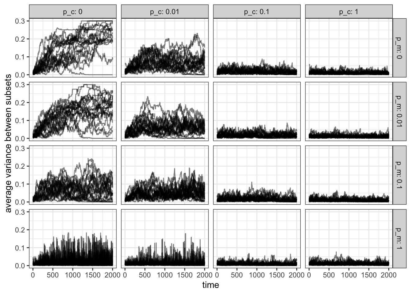

In the absence of contact and migration ($p_m=p_c=0$) the variance is highest between subsets. The variance decreases more quickly as $p_c$ increases compared to $p_m$.

Figure 15.11: In the absence of contact and migration ($p_m=p_c=0$) the variance is highest between subsets. The variance decreases more quickly as $p_c$ increases compared to $p_m$.

In accordance with our previous results in the absence of migration and contact the variance is highest, whereas it is lowest when both $p_m$ and $p_c$ are 1. However, we also see that variance drops faster as $p_c$ increases compared to the same increase in $p_m$ (compare $p_c=0.1, p_m=0$ and $p_c=0, p_m=0.1$).

Sometimes we will not have the space to plot a grid like this. In that case, we could condense the results further down by averaging, say, the last $20\%$ of the simulation rounds overall simulations and then plot a single value for each parameter pair. A good visualisation for this is the raster, which ggplot provides with the geom_raster() function.

But first, we need to summarise our data using the following tidyverse functions: we use filter() to select only the rows of the last $20\%$ of our simulation turns, handing this over (%>%) to the group_by() function, which will create groups where p_m and p_c are identical, and then summarise(), which will add a new column with the average var values from our results object. We will store the summarised result in res_summ:

res_summ <- filter(res, time >= (max(time)*.8)) %>% 
              group_by(p_m, p_c) %>% 
                summarise(mean_var = mean(var), .groups = "keep")

We can now use res_summ to plot our raster where we set the z-value (the colour of each raster rectangle) using the fill argument:

ggplot(res_summ) +
  geom_raster(aes(x = factor(p_m), y = factor(p_c), fill = mean_var)) +
  xlab("p_m") + ylab("p_c") + 
  theme_bw() +
  theme(legend.title = element_blank())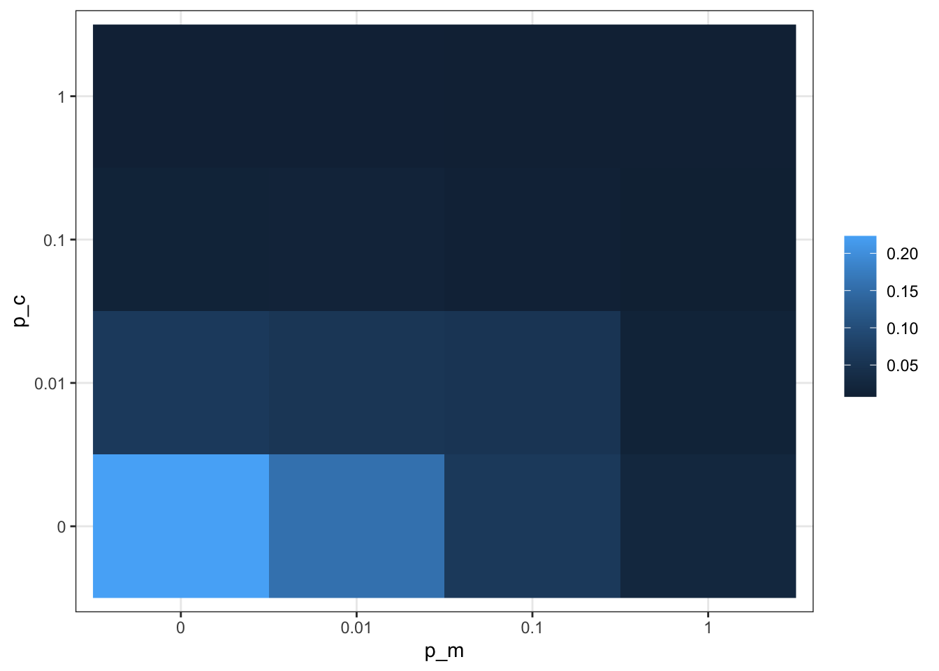

Summarised simulation results showing the effect of contact and migration on the distribution of behaviour 1 among subsets of a population.

Figure 15.12: Summarised simulation results showing the effect of contact and migration on the distribution of behaviour 1 among subsets of a population.

Our results show that contact and migration are not interchangeable or symmetric in their behaviour. With this model, we could now ask many more interesting questions, for example, how migration and contact probability affect trait distribution in populations with unevenly sized subsets, or how the number of clusters, behaviours, or population size affects the results. Below, we have a selection of further model extensions to consider.

15.5 Summary of the model

In this chapter, we have used a simple model to simulate the effect of population sub-structuring. We have seen how contact (movement of cultural traits) and migration (movement of individuals) affect the frequency of a behaviour in each subset. When migration and contact probability are low, the frequency of individual behaviours become uncorrelated between subsets. However, as both parameters increase, subsets behave more and more like a single large population. This means that depending on the rate of contact and migration, sub-structuring can have different effects on cultural dynamics.

15.6 Further reading

There are a few interesting empirical studies on migration and the social transmission of locally adaptive behaviours in animals. For example, the study by Luncz and Boesch (2014) reports on the stability of tool traditions in neighbouring chimpanzee communities. There are also a few theoretical studies on the persistence or change of local traditions. Boyd and Richerson (2009), for example, focus on how adaptive a behaviour is, whereas Mesoudi (2018) focuses on the strength of acculturation that is required to maintain cultural diversity between groups.