Chapter 4 Biased transmission: frequency-dependent indirect bias
In Chapter 3 we looked at the case where one cultural trait is intrinsically more likely to be copied than another trait. Here we will start looking at the other kind of biased transmission when traits are equivalent, but individuals are more likely to adopt a trait according to the characteristics of the population, and in particular which other individuals already have it. (As we mentioned previously, these are often called ‘indirect’ or ‘context’ biases).
4.1 The logic of conformity
A first possibility is that we may be influenced by the frequency of the trait in the population, i.e. how many other individuals already have the trait. Conformity (or ‘positive frequency-dependent bias’) has been most studied. Here, individuals are disproportionately more likely to adopt the most common trait in the population, irrespective of its intrinsic characteristics. (The opposite case, anti-conformity or negative frequency-dependent bias is also possible, where the least common trait is more likely to be copied. This is probably less common in real life.)
For example, imagine trait \(A\) has a frequency of 0.7 in the population, with the rest possessing trait \(B\). An unbiased learner would adopt trait \(A\) with a probability exactly equal to 0.7. This is unbiased transmission and is what happens the model described in Chapter 1 by picking a member of the previous generation at random, the probability of adoption is equal to the frequency of that trait among the previous generation.
A conformist learner, on the other hand, would adopt trait \(A\) with a probability greater than 0.7. In other words, common traits get an ‘adoption boost’ relative to unbiased transmission. Uncommon traits get an equivalent ‘adoption penalty.’ The magnitude of this boost or penalty can be controlled by a parameter, which we will call \(D\).
Let’s keep things simple in our model. Rather than assuming that individuals sample across the entire population, which in any case might be implausible in large populations, let’s assume they pick only three demonstrators at random. Why three? This is the minimum number of demonstrators that can yield a majority (i.e. 2 vs 1), which we need to implement conformity. When two demonstrators have one trait and the other demonstrator has a different trait, we want to boost the probability of adoption for the majority trait, and reduce it for the minority trait.
We can specify the probability of adoption as follows:
Table 1: Probability of adopting trait \(A\) for each possible combination of traits amongst three demonstrators
| Demonstrator 1 | Demonstrator 2 | Demonstrator 3 | Probability of adopting trait \(A\) |
|---|---|---|---|
| \(A\) | \(A\) | \(A\) | 1 |
| \(A\) | \(A\) | \(B\) | \(2/3 + D/3\) |
| \(A\) | \(B\) | \(A\) | \(2/3 + D/3\) |
| \(B\) | \(A\) | \(A\) | \(2/3 + D/3\) |
| \(A\) | \(B\) | \(B\) | \(1/3 - D/3\) |
| \(B\) | \(A\) | \(B\) | \(1/3 - D/3\) |
| \(B\) | \(B\) | \(A\) | \(1/3 - D/3\) |
| \(B\) | \(B\) | \(B\) | 0 |
The first row says that when all demonstrators have trait \(A\), then trait \(A\) is definitely adopted. Similarly, the bottom row says that when all demonstrators have trait \(B\), then trait \(A\) is never adopted, and by implication trait \(B\) is always adopted.
For the three combinations where there are two \(A\)s and one \(B\), the probability of adopting trait \(A\) is \(2/3\), which it would be under unbiased transmission (because two out of three demonstrators have \(A\)), plus the conformist adoption boost specified by \(D\). As we want \(D\) to vary from 0 to 1, it is divided by three, so that the maximum probability of adoption is equal to 1 (when \(D=1\)).
Similarly, for the three combinations where there are two \(B\)s and one \(A\), the probability of adopting \(A\) is \(1/3\) minus the conformist adoption penalty specified by \(D\).
Let’s implement these assumptions in the kind of individual-based model we’ve been building so far. As before, assume \(N\) individuals each of whom possesses one of two traits \(A\) or \(B\). The frequency of \(A\) is denoted by \(p\). The initial frequency of \(A\) in generation \(t=1\) is \(p_0\). Rather than going straight to a function, let’s go step by step.
First, we’ll specify our parameters, \(N\) and \(p_0\) as before, plus the new conformity parameter \(D\). We also create the usual population tibble and fill it with \(A\)s and \(B\)s in the proportion specified by \(p_0\), again exactly as before.
library(tidyverse)

N <- 100
p_0 <- 0.5
D <- 1

# Create first generation
population <- tibble(trait = sample(c("A", "B"), N,
                                    replace = TRUE, prob = c(p_0, 1 - p_0)))
Now we create another tibble called demonstrators that picks, for each new individual in the next generation, three demonstrators at random from the current population of individuals. It therefore needs three columns/variables, one for each of the demonstrators, and \(N\) rows, one for each individual. We fill each column with randomly chosen traits from thepopulation tibble. We can have a look at demonstrators by entering its name in the R console.
# Create a tibble with a set of 3 randomly-picked demonstrators for each agent
demonstrators <- tibble(dem1 = sample(population$trait, N, replace = TRUE),
                        dem2 = sample(population$trait, N, replace = TRUE),
                        dem3 = sample(population$trait, N, replace = TRUE))

# Visualise the tibble
demonstrators
## # A tibble: 100 x 3
## dem1 dem2 dem3
## <chr> <chr> <chr>
## 1 B B B
## 2 B A B
## 3 B B A
## 4 B A A
## 5 A B B
## 6 A A B
## 7 B B B
## 8 B B A
## 9 B B B
## 10 A B B
## # … with 90 more rowsThink of each row here as containing the traits of three randomly-chosen demonstrators chosen by each new next-generation individual. Now we want to calculate the probability of adoption of \(A\) for each of these three-trait demonstrator combinations.
First we need to get the number of \(A\)s in each combination. Then we can replace the traits in population based on the probabilities in Table 1. When all demonstrators have \(A\), we set to \(A\). When no demonstrators have \(A\), we set to \(B\). When two out of three demonstrators have \(A\), we set to \(A\) with probability \(2/3 + D/3\) and \(B\) otherwise. When one out of three demonstrators have \(A\), we set to \(A\) with probability \(1/3 - D/3\) and \(B\) otherwise.
# Get the number of As in each 3-demonstrator combinations
num_As <- rowSums(demonstrators == "A")

# For 3-demonstrator combinations with all As, set to A
population$trait[num_As == 3] <- "A"
# For 3-demonstrator combinations with all Bs, set to B
population$trait[num_As == 0] <- "B"

prob_majority <- sample(c(TRUE, FALSE),
                        prob = c((2/3 + D/3), 1 - (2/3 + D/3)), N, replace = TRUE)
prob_minority <- sample(c(TRUE, FALSE),
                        prob = c((1/3 - D/3), 1 - (1/3 - D/3)), N, replace = TRUE)

# 3-demonstrator combinations with two As and one B
if (nrow(population[prob_majority & num_As == 2, ]) > 0) {
  population[prob_majority & num_As == 2, ]$trait <- "A"
}
if (nrow(population[prob_majority == FALSE & num_As == 2, ]) > 0) {
  population[prob_majority == FALSE & num_As == 2, ]$trait <- "B"
}

# 3-demonstrator combinations with one A and two Bs
if (nrow(population[prob_minority & num_As == 1, ]) > 0) {
  population[prob_minority & num_As == 1, ]$trait <- "A"
}
if (nrow(population[prob_minority == FALSE & num_As == 1, ]) > 0) {
  population[prob_minority == FALSE & num_As == 1, ]$trait <- "B"
}
To check it works, we can add the new population tibble as a column to demonstrators and have a look at it. This will let us see the three demonstrators and the resulting new trait side by side.
demonstrators <- add_column(demonstrators, new_trait = population$trait)

# Visualise the tibble
demonstrators
## # A tibble: 100 x 4
## dem1 dem2 dem3 new_trait
## <chr> <chr> <chr> <chr>
## 1 B B B B
## 2 B A B B
## 3 B B A B
## 4 B A A A
## 5 A B B B
## 6 A A B A
## 7 B B B B
## 8 B B A B
## 9 B B B B
## 10 A B B B
## # … with 90 more rowsBecause we set \(D=1\) above, the new trait is always the majority trait among the three demonstrators. This is perfect conformity. We can weaken conformity by reducing \(D\). Here is an example with \(D=0.5\). All the code is the same as what we already discussed above.
D <- 0.5

# create first generation
population <- tibble(trait = sample(c("A", "B"), N,
                                    replace = TRUE, prob = c(p_0, 1 - p_0)))

# Create a tibble with a set of 3 randomly-picked demonstrators for each agent
demonstrators <- tibble(dem1 = sample(population$trait, N, replace = TRUE),
                        dem2 = sample(population$trait, N, replace = TRUE),
                        dem3 = sample(population$trait, N, replace = TRUE))

# Get the number of As in each 3-demonstrator combinations
num_As <- rowSums(demonstrators == "A")

# For 3-demonstrator combinations with all As, set to A
population$trait[num_As == 3] <- "A"
# For 3-demonstrator combinations with all Bs, set to B
population$trait[num_As == 0] <- "B"

prob_majority <- sample(c(TRUE, FALSE),
                        prob = c((2/3 + D/3), 1 - (2/3 + D/3)), N, replace = TRUE)
prob_minority <- sample(c(TRUE, FALSE),
                        prob = c((1/3 - D/3), 1 - (1/3 - D/3)), N, replace = TRUE)

# 3-demonstrator combinations with two As and one B
if (nrow(population[prob_majority & num_As == 2, ]) > 0) {
  population[prob_majority & num_As == 2, ]$trait <- "A"
}
if (nrow(population[prob_majority == FALSE & num_As == 2, ]) > 0) {
  population[prob_majority == FALSE & num_As == 2, ]$trait <- "B"
}

# 3-demonstrator combinations with one A and two Bs
if (nrow(population[prob_minority & num_As == 1, ]) > 0) {
  population[prob_minority & num_As == 1, ]$trait <- "A"
}
if (nrow(population[prob_minority == FALSE & num_As == 1, ]) > 0) {
  population[prob_minority == FALSE & num_As == 1, ]$trait <- "B"
}

demonstrators <- add_column(demonstrators, new_trait = population$trait)

# Visualise the tibble
demonstrators
## # A tibble: 100 x 4
## dem1 dem2 dem3 new_trait
## <chr> <chr> <chr> <chr>
## 1 A B A A
## 2 A A B A
## 3 B A A B
## 4 B B B B
## 5 A B B B
## 6 A B A B
## 7 B A B B
## 8 B A B B
## 9 B A B B
## 10 B A A A
## # … with 90 more rowsNow that conformity is weaker, sometimes the new trait is not the majority amongst the three demonstrators.
4.2 Testing conformist transmission
As in the previous chapters, we can put all this code together into a function to see what happens over multiple generations and in multiple runs. There is nothing new in the code below, which is a combination of the code we already wrote in Chapter 1 and the new bits of code for conformity introduced above.
conformist_transmission <- function (N, p_0, D, t_max, r_max) {

  output <- tibble(generation = rep(1:t_max, r_max),
                   p = as.numeric(rep(NA, t_max * r_max)),
                   run = as.factor(rep(1:r_max, each = t_max)))

  for (r in 1:r_max) {
    # Create first generation
    population <- tibble(trait = sample(c("A", "B"), N,
                                        replace = TRUE, prob = c(p_0, 1 - p_0)))

    # Add first generation's p for run r
    output[output$generation == 1 & output$run == r, ]$p <-
      sum(population$trait == "A") / N

    for (t in 2:t_max) {

      # Create a tibble with a set of 3 randomly-picked demonstrators for each agent
      demonstrators <- tibble(dem1 = sample(population$trait, N, replace = TRUE),
                              dem2 = sample(population$trait, N, replace = TRUE),
                              dem3 = sample(population$trait, N, replace = TRUE))

      # Get the number of As in each 3-demonstrator combinations
      num_As <- rowSums(demonstrators == "A")

      # For 3-demonstrator combinations with all As, set to A
      population$trait[num_As == 3] <- "A"
      # For 3-demonstrator combinations with all Bs, set to B
      population$trait[num_As == 0] <- "B"

      prob_majority <- sample(c(TRUE, FALSE),
                              prob = c((2/3 + D/3), 1 - (2/3 + D/3)), N, replace = TRUE)
      prob_minority <- sample(c(TRUE, FALSE),
                              prob = c((1/3 - D/3), 1 - (1/3 - D/3)), N, replace = TRUE)

      # 3-demonstrator combinations with two As and one B
      if (nrow(population[prob_majority & num_As == 2, ]) > 0) {
        population[prob_majority & num_As == 2, ]$trait <- "A"
      }
      if (nrow(population[prob_majority == FALSE & num_As == 2, ]) > 0) {
        population[prob_majority == FALSE & num_As == 2, ]$trait <- "B"
      }
      # 3-demonstrator combinations with one A and two Bs
      if (nrow(population[prob_minority & num_As == 1, ]) > 0) {
        population[prob_minority & num_As == 1, ]$trait <- "A"
      }
      if (nrow(population[prob_minority == FALSE & num_As == 1, ]) > 0) {
        population[prob_minority == FALSE & num_As == 1, ]$trait <- "B"
      }

      # Get p and put it into output slot for this generation t and run r
      output[output$generation == t & output$run == r, ]$p <-
        sum(population$trait == "A") / N
    }
  }
  # Export data from function
  output
}
We can test the function with perfect conformity (\(D=1\)) and plot it (again we use the function plot_multiple_runs() we wrote in Chapter 1).
data_model <- conformist_transmission(N = 1000, p_0 = 0.5, D = 1, t_max = 50, r_max = 10)
plot_multiple_runs(data_model)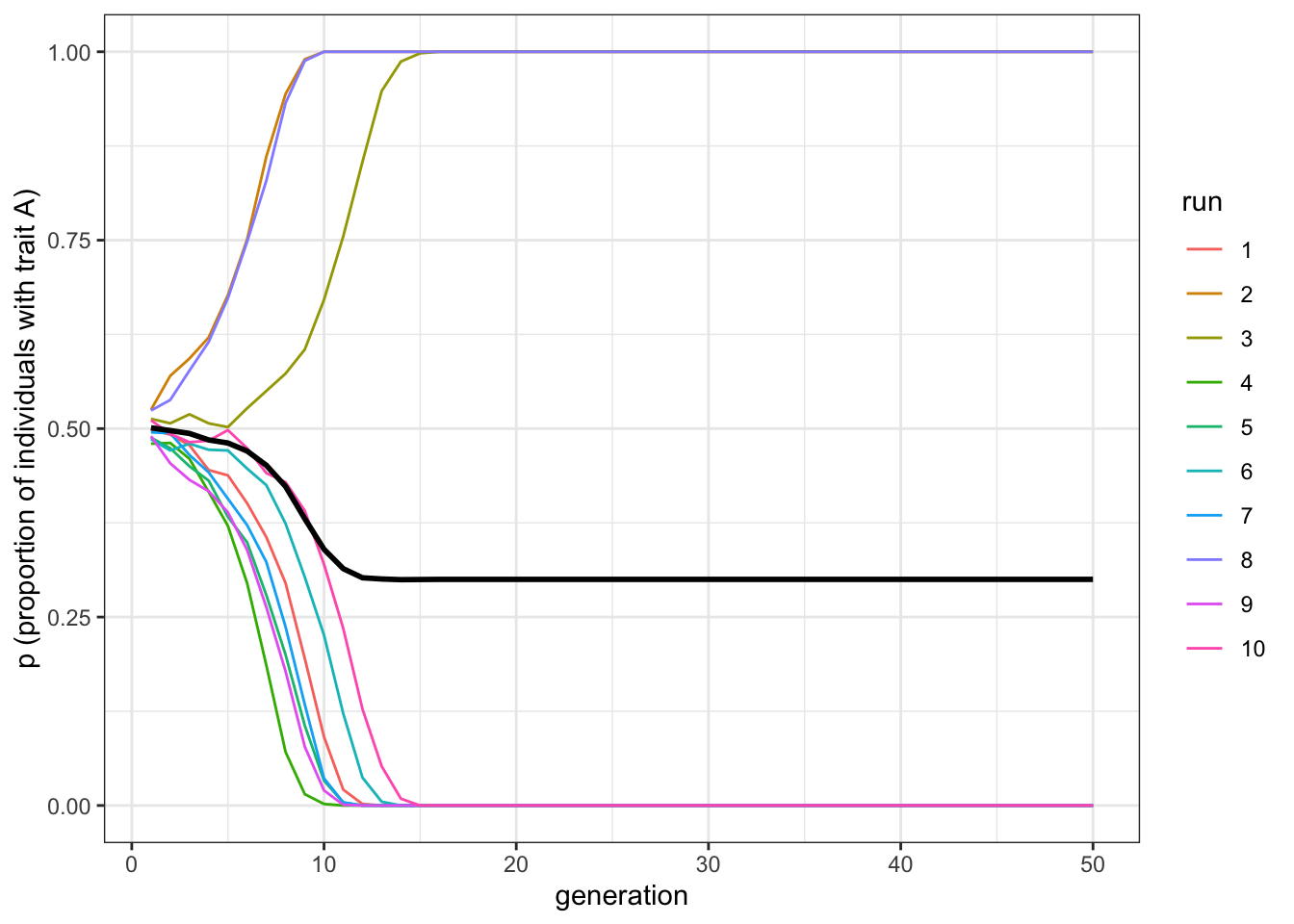
Figure 4.1: Conformity causes one trait to spread and replace the other by favouring whichever trait is initially most common
Here we should see some lines going to \(p=1\), and some lines going to \(p=0\). Conformity acts to favour the majority trait. This will depend on the initial frequency of \(A\) in the population. In different runs with \(p_0=0.5\), sometimes there will be slightly more \(A\)s, sometimes slightly more \(B\)s (remember, in our model, this is probabilistic, like flipping coins, so initial frequencies will rarely be precisely 0.5).
What happens if we set \(D=0\)?
data_model <- conformist_transmission(N = 1000, p_0 = 0.5, D = 0, t_max = 50, r_max = 10)
plot_multiple_runs(data_model)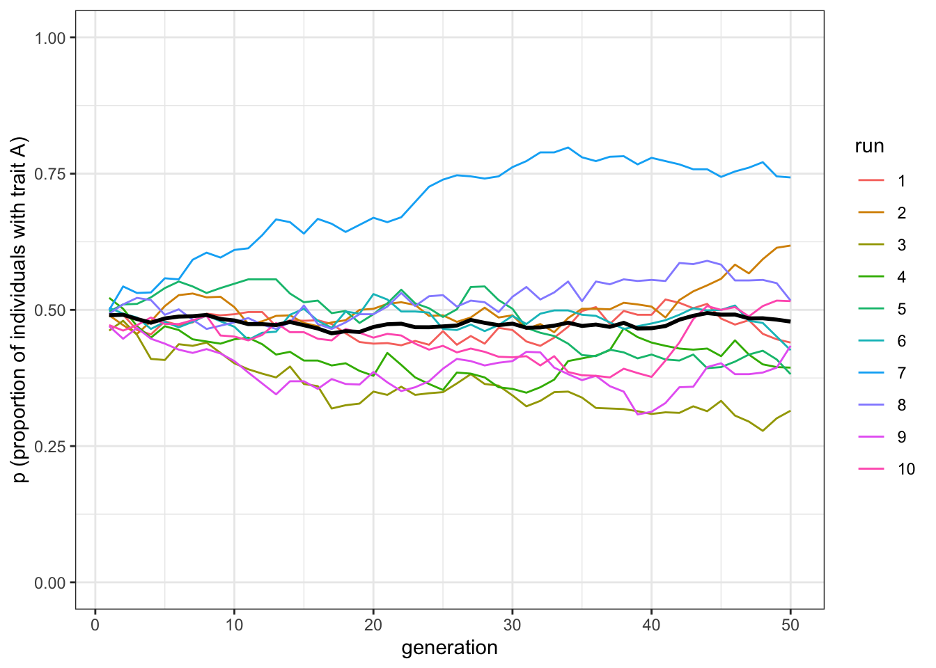
Figure 4.2: Removing conformist bias recreates unbiased transmission, and does not systematically change trait frequencies
This model is equivalent to unbiased transmission. As for the simulations described in Chapter 1, with a sufficiently large \(N\), the frequencies fluctuate around \(p=0.5\). This underlines the effect of conformity. With unbiased transmission, majority traits are favoured because they are copied in proportion to their frequency (incidentally, it is for this reason that ‘copying the majority’ is not a good description of conformity in the technical sense used in the field of cultural evolution: even with unbiased copying the majority trait is copied more than the minority one). However, they reach fixation only in small populations. With conformity, instead, the majority trait is copied with a probability higher than its frequency, so that conformity drives traits to fixation as they become more and more common.
As an aside, note that the last two graphs have roughly the same thick black mean frequency line, which hovers around \(p=0.5\). This highlights the dangers of looking at means alone. If we hadn’t plotted the individual runs and relied solely on mean frequencies, we might think that \(D=0\) and \(D=1\) gave identical results. But in fact, they are very different. Always look at the underlying distribution that generates means.
Now let’s explore the effect of changing the initial frequencies by changing \(p_0\), and adding conformity back in.
data_model <- conformist_transmission(N = 1000, p_0 = 0.55, D = 1, t_max = 50, r_max = 10)
plot_multiple_runs(data_model)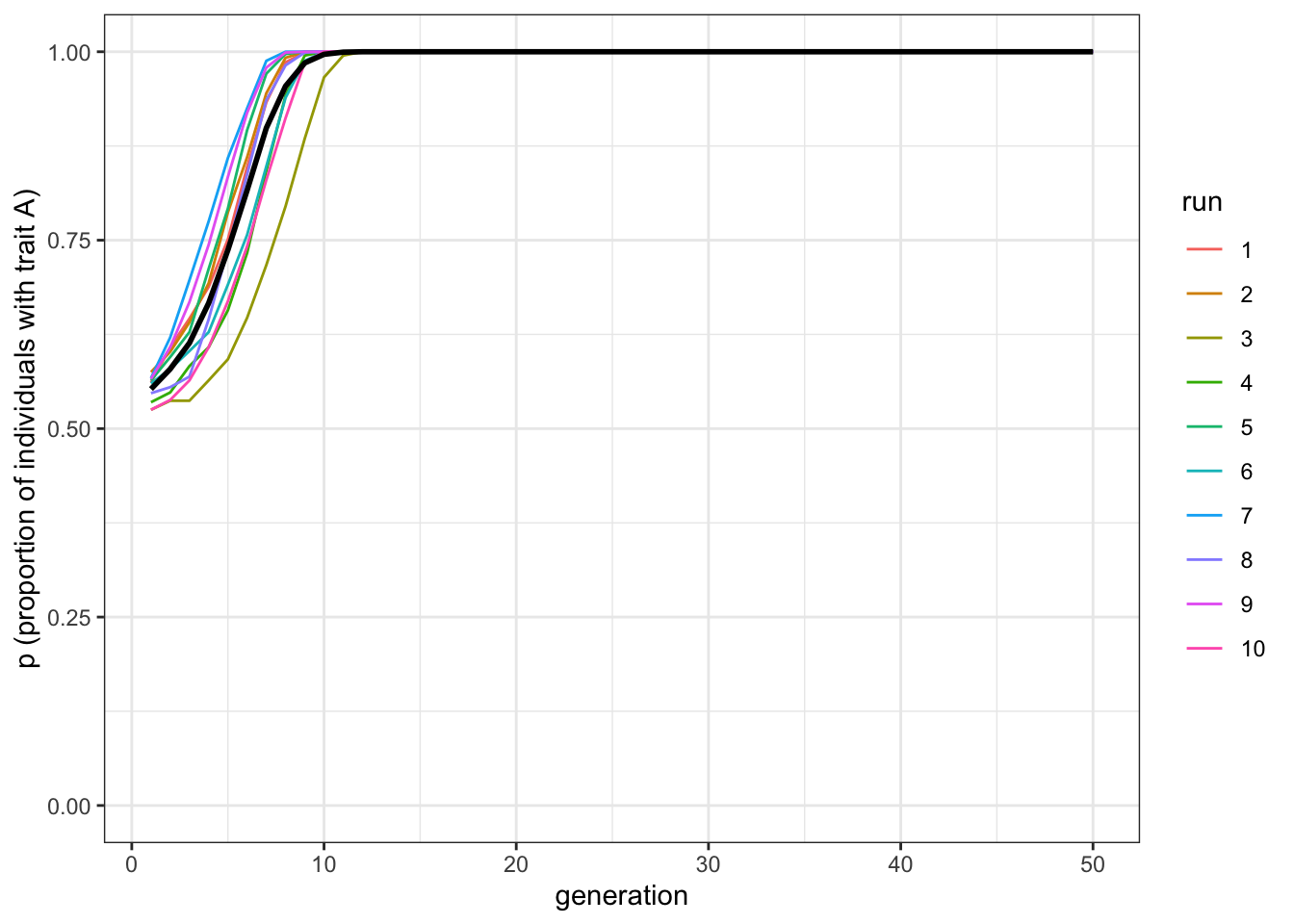
Figure 4.3: When trait A is always initially in the majority, it is always favoured by conformity
When \(A\) starts with a slight majority (\(p_0=0.55\)), all (or almost all) of the runs result in \(A\) going to fixation. Now let’s try the reverse.
data_model <- conformist_transmission(N = 1000, p_0 = 0.45, D = 1, t_max = 50, r_max = 10)
plot_multiple_runs(data_model)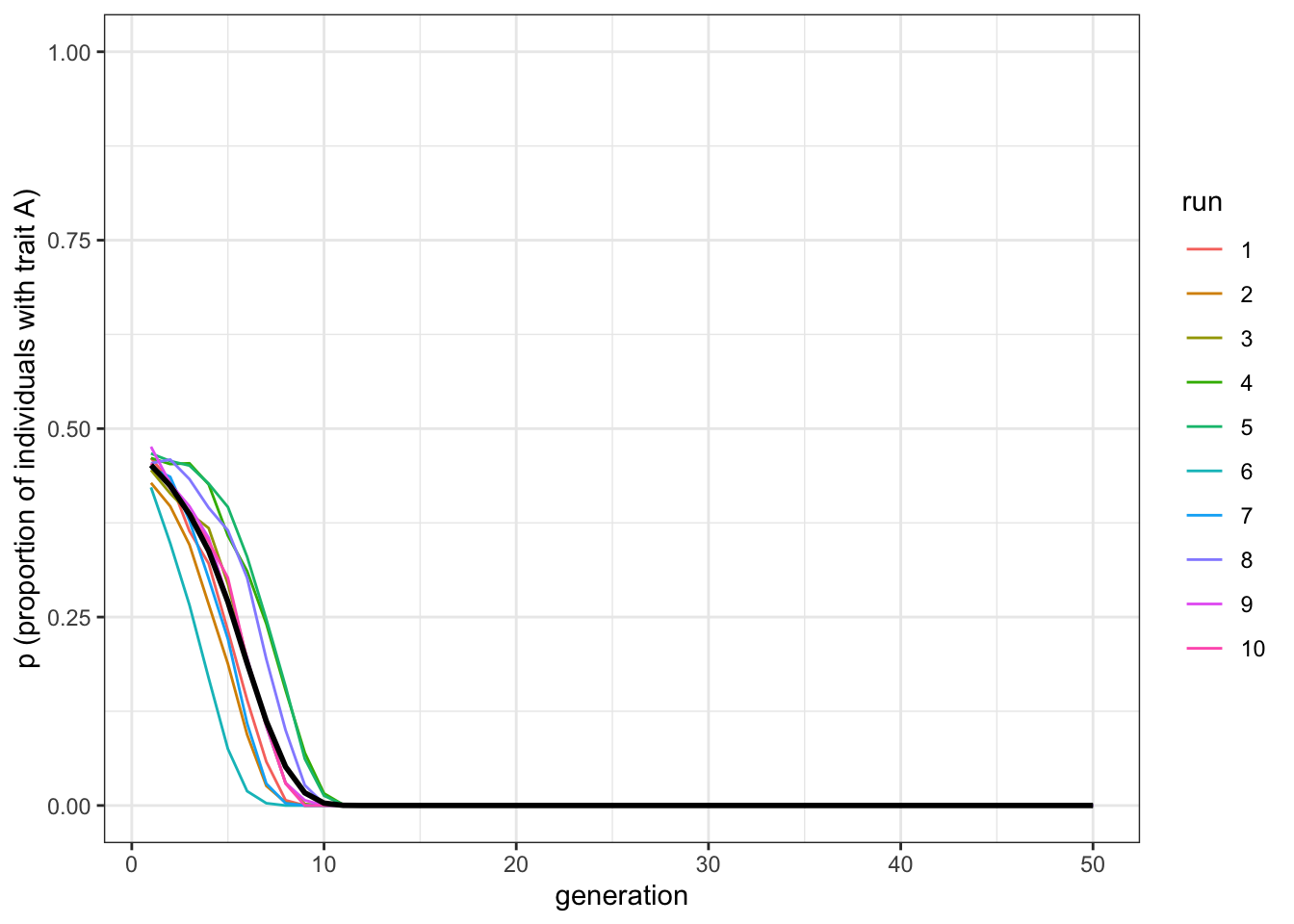
Figure 4.4: When trait B is always initially in the majority, it is always favoured by conformity
When \(A\) starts off in a minority (\(p_0=0.45\)), all (or almost all) of the runs result in \(A\) disappearing. These last two graphs show how initial conditions affect conformity. Whichever trait is more common is favoured by conformist transmission.
4.3 Summary of the model
In this chapter, we explored conformist biased cultural transmission. This is where individuals are disproportionately more likely to adopt the most common trait among a set of demonstrators. We can contrast this indirect bias with the direct (or content) biased transmission from [Chapter 3][Biased transmission (direct bias)], where one trait is intrinsically more likely to be copied. With conformity, the traits have no intrinsic difference in attractiveness and are preferentially copied simply because they are common.
We saw how conformity increases the frequency of whichever trait is more common. Initial trait frequencies are important here: traits that are initially more common typically go to fixation. This, in turn, makes stochasticity important, which in small populations can affect initial frequencies.
We also discussed the subtle but fundamental difference between unbiased copying and conformity. In both, majority traits are favoured, but it is only with conformity that they are disproportionately favoured. In large populations, unbiased transmission rarely leads to trait fixation, whereas conformist transmission often does. Furthermore, as we will see later, conformity also makes majority traits resistant to external disturbances, such as the introduction of other traits via innovation or migration.
4.4 Further readings
Boyd and Richerson (1985) introduced conformist or positive frequency-dependent cultural transmission as defined here, and modelled it analytically with similar methods. Henrich and Boyd (1998) modelled the evolution of conformist transmission, while Efferson et al. (2008) provided experimental evidence that at least some people conform in a simple learning task.