Chapter 1 Unbiased transmission
We start by simulating a simple case of unbiased cultural transmission. We will detail each step of the simulation and explain the code line-by-line. In the following chapters, we will reuse most of this initial model, building up the complexity of our simulations.
1.1 Initialising the simulation
Here we will simulate a case where each of \(N\) individuals possesses one of two mutually exclusive cultural traits. We denote these alternative traits as \(A\) and \(B\). For example, \(A\) might be eating a vegetarian diet, and \(B\) might be eating a non-vegetarian diet. In reality, traits are seldom as clear-cut (e.g. what about pescatarians?), but models are designed to cut away all the complexity to give tractable answers to simplified situations.
Our model has non-overlapping generations. That is, in each generation all \(N\) individuals die and are replaced with \(N\) new individuals. Again, this is an extreme but common assumption in evolutionary models. It provides a simple way of simulating change over time. Generations here could correspond to biological generations, but could equally be ‘cultural generations’ (or learning episodes).
Each new individual of each new generation picks a member of the previous generation at random and copies their cultural trait. This is known as unbiased oblique cultural transmission. It is unbiased because traits are copied entirely at random. The term oblique means that members of one generation learn from those of the previous, non-overlapping, generation. This is different from, for example, horizontal cultural transmission, where individuals copy members of the same generation, and vertical cultural transmission, where offspring copy their biological parents.
Given the two traits \(A\) and \(B\) and an unbiased oblique cultural transmission, how is their average frequency in the population going to change over time? To answer this question, we need to keep track of the frequency of both traits. We will use \(p\) to indicate the proportion of the population with trait \(A\), which is simply the number of all individuals with trait \(A\) divided by the number of all individuals, \(p=\frac{n_A}{N}\). Because we only have two mutually exclusive traits in our population, we know that the proportion of individuals with trait \(B\) must be \((1-p)\). For example, if \(70\%\) of the population have trait \(A\) \((p=0.7)\), then the remaining \(30\%\) must have trait \(B\) (i.e. \(1-p=1-0.7=0.3\)).
The output of the model will be a plot showing \(p\) over all generations up to the last generation. Generations (or time steps) are denoted by \(t\), where generation one is \(t=1\), generation two is \(t=2\), up to the last generation \(t=t_{\text{max}}\).
First, we need to specify the fixed parameters of the model. These are quantities that we decide on at the start and do not change during the simulation. In this model, these are N (the number of individuals) and t_max (the number of generations). Let’s start with N = 100 and t_max = 200:
N <- 100
t_max <- 200
Now we need to create our individuals. The only information we need to keep about our individuals is their cultural trait (\(A\) or \(B\)). We’ll call population the data structure containing the individuals. The type of data structure we have chosen here is a tibble. This is a more user-friendly version of a data.frame. Tibbles, and the tibble command, are part of the tidyverse library, which we need to call before creating the tibble. We will use other commands from the tidyverse throughout the book.
Initially, we’ll give each individual either an \(A\) or \(B\) at random, using the sample() command. This can be seen in the code chunk below. The sample() command takes three arguments (i.e. inputs or options). The first argument lists the elements to pick at random, in our case, the traits \(A\) and \(B\). The second argument gives the number of times to pick, in our case \(N\) times, once for each individual. The final argument says to replace or reuse the elements specified in the first argument after they’ve been picked (otherwise there would only be one copy of \(A\) and one copy of \(B\), so we could only assign traits to two individuals before running out). Within the tibble command, the word trait denotes the name of the variable within the tibble that contains the random \(A\)s and \(B\)s, and the whole tibble is assigned the name population.
library(tidyverse)
population <- tibble(trait = sample(c("A", "B"), N, replace = TRUE))
We can see the cultural traits of our population by simply entering its name in the R console:
population## # A tibble: 100 x 1
## trait
## <chr>
## 1 B
## 2 A
## 3 B
## 4 B
## 5 A
## 6 B
## 7 A
## 8 A
## 9 B
## 10 A
## # … with 90 more rowsAs expected, there is a single column called trait containing \(A\)s and \(B\)s. The type of the column, in this case <chr> (i.e. character), is reported below the name.
A specific individual’s trait can be retrieved using the square bracket notation in R. For example, individual 4’s trait can be retrieved by typing:
population$trait[4]## [1] "B"This matches the fourth row in the table above.
We also need a tibble to record the output of our simulation, that is, to track the trait frequency \(p\) in each generation. This will have two columns with \(t_{\text{max}}\) rows, one row for each generation. The first column is simply a counter of the generations, from 1 to \(t_{\text{max}}\). This will be useful for plotting the output later. The other column should contain the values of \(p\) for each generation.
At this stage we don’t know what \(p\) will be in each generation, so for now let’s fill the output tibble with ‘NA’s, which is R’s symbol for Not Available, or missing value. We can use the rep() (repeat) command to repeat ’NA’ \(t_{\text{max}}\) times. We’re using ‘NA’ rather than, say, zero, because zero could be misinterpreted as \(p=0\), which would mean that all individuals have trait \(B\). This would be misleading, because at the moment we haven’t yet calculated \(p\), so it’s non-existent, rather than zero.
output <- tibble(generation = 1:t_max, p = rep(NA, t_max))We can, however, fill in the first value of p for our already-created first generation of individuals, held in population. The command below sums the number of \(A\)s in population and divides it by \(N\) to get a proportion rather than an absolute number. It then puts this proportion in the first slot of p in output, the one for the first generation, \(t=1\). We can again write the name of the tibble, output, to see that it worked.
output$p[1] <- sum(population$trait == "A") / N
output
## # A tibble: 200 x 2
## generation p
## <int> <dbl>
## 1 1 0.4
## 2 2 NA
## 3 3 NA
## 4 4 NA
## 5 5 NA
## 6 6 NA
## 7 7 NA
## 8 8 NA
## 9 9 NA
## 10 10 NA
## # … with 190 more rowsThis first value of p will be close to \(0.5\), meaning that around 50 individuals have trait \(A\), and 50 have trait \(B\). Even though sample() returns either trait with equal probability, this does not necessarily mean that we will get exactly 50 \(A\)s and 50 \(B\)s. This happens with simulations and finite population sizes: they are probabilistic (or stochastic), not deterministic. Analogously, flipping a coin 100 times will not always give exactly 50 heads and 50 tails. Sometimes we will get 51 heads, sometimes 49, etc. To see this in our simulation, you can re-run all of the above code and you will get a different \(p\).
1.2 Execute generation turn-over many times
Now that we set up the population, we can simulate what individuals do in each generation. We iterate these actions over \(t_{\text{max}}\) generations. In each generation, we will:
copy the current individuals to a separate tibble called
previous_populationto use as demonstrators for the new individuals; this allows us to implement oblique transmission with its non-overlapping generations, rather than mixing up the generationscreate a new generation of individuals, each of whose trait is picked at random from the
previous_populationtibblecalculate \(p\) for this new generation and store it in the appropriate slot in
output
To iterate, we’ll use a for-loop, using t to track the generation. We’ve already done generation 1 so we’ll start at generation 2. The random picking of models is done with sample() again, but this time picking from the traits held in previous_population. Note that we have added comments briefly explaining what each line does. This is perhaps superfluous when the code is this simple, but it’s always good practice. Code often growths organically. As code pieces get cut, pasted, and edited, they can lose their context. Explaining what each line does lets other people - and a future, forgetful you - know what’s going on.
for (t in 2:t_max) {
  # Copy the population tibble to previous_population tibble
  previous_population <- population

  # Randomly copy from previous generation's individuals
  population <- tibble(trait = sample(previous_population$trait, N, replace = TRUE))

  # Get p and put it into the output slot for this generation t
  output$p[t] <- sum(population$trait == "A") / N
}
Now we should have 200 values of p stored in output, one for each generation. You can list them by typing output, but more effective is to plot them.
1.3 Plotting the model results
We use ggplot() to plot our data. The syntax of ggplot may be slightly obscure at first, but it forces us to have a clear picture of the data before plotting.
In the first line in the code below, we are telling ggplot that the data we want to plot is in the tibble output. Then, with the command aes(), we declare the ‘aesthetics’ of the plot, that is, how we want our data mapped in our plot. In this case, we want the values of p on the y-axis, and the values of generation on the x-axis (this is why we created a column in the output tibble, to keep the count of generations).
We then use geom_line(). In ggplot, ‘geoms’ describe what kind of visual representation should be plotted: lines, bars, boxes and so on. This visual representation is independent of the mapping that we declared before with aes(). The same data, with the same mapping, can be visually represented in many different ways. In this case, we are telling ggplot to plot the data as a line graph. You can change geom_line() in the code below to geom_point() to turn the graph into a scatter plot (there are many more geoms and we will see some of them in later chapters).
The remaining commands are mainly to make the plot look nicer. For example, with ylim we set the y-axis limits to be between 0 and 1, i.e. all the possible values of \(p\). We also use one of the basic black and white themes(theme_bw), which looks more professional than the generic ggplot theme.ggplot automatically labels the axis with the name of the tibble columns that are plotted. With the command labs() we provide a more informative label for the y-axis.
ggplot(data = output, aes(y = p, x = generation)) +
  geom_line() +
  ylim(c(0, 1)) +
  theme_bw() +
  labs(y = "p (proportion of individuals with trait A)")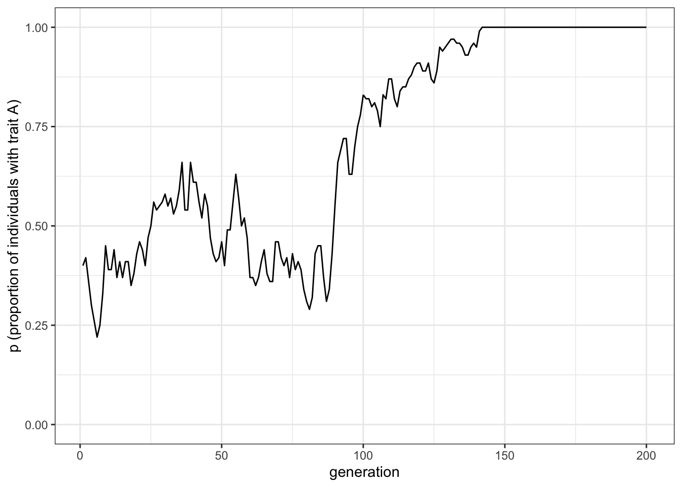
Figure 1.1: Random fluctuations of the proportion of trait A under unbiased cultural transmission
Unbiased transmission, or random copying, is by definition random. Hence, different runs of our simulation will generate different plots. If you rerun all the code you will get something different. In all cases, the proportion of individuals with trait \(A\) start around 0.5 and then oscillate stochastically. Occasionally, \(p\) will reach and then stay at 0 or 1. At \(p = 0\) there are no \(A\)s and every individual possesses \(B\). At \(p=1\) there are no \(B\)s and every individual possesses \(A\). This is a typical feature of cultural drift. Analogous to genetic drift we find that in small populations and in the absence of migration and mutation (or innovation in the case of cultural evolution) traits can be lost purely by chance after some generations.
1.4 Write a function to wrap the model code
What would happen if we increase population size \(N\)? Are we more or less likely to lose one of the traits? Ideally, we would like to repeat the simulation to explore this idea in more detail. As noted above, individual-based models like this one are probabilistic (or stochastic), thus it is essential to run simulations many times to understand what happens. With our code scattered about in chunks, it is hard to quickly repeat the simulation. Instead, we can wrap it all up in a function:
unbiased_transmission_1 <- function(N, t_max) {
  population <- tibble(trait = sample(c("A", "B"), N, replace = TRUE))
  output <- tibble(generation = 1:t_max, p = rep(NA, t_max))
  output$p[1] <- sum(population$trait == "A") / N
  for (t in 2:t_max) {
    # Copy individuals to previous_population tibble
    previous_population <- population

    # Randomly copy from previous generation
    population <- tibble(trait = sample(previous_population$trait, N, replace = TRUE))

    # Get p and put it into output slot for this generation t
    output$p[t] <- sum(population$trait == "A") / N
  }
  # Export data from function
  output
}
With the function() function we tell R to run several lines of code that are enclosed in the two curly braces. Additionally, we declare two arguments that we will hand over whenever we execute the function, here N and t_max. As you can see we have used the same code snippets that we already ran above. In addition, unbiased_transmission_1() ends with the line output. This means that this tibble will be exported from the function when it is run. This is useful for storing data from simulations wrapped in functions, otherwise, that data is lost after the function is executed.
When you run the above code there will be no output in the terminal. All you have done is define the function and not actually run it. We just told R what to do, when we call the function. Now we can easily change the values of \(N\) and \(t_{\text{max}}\). Let’s first try the same values of \(N\) and \(t_{\text{max}}\) as before, and save the output from the simulation into data_model.
data_model <- unbiased_transmission_1(N = 100, t_max = 200)Let us also create a function to plot the data, so we do not need to rewrite all the plotting instructions each time. While this may seem impractical now, it is convenient to separate the function that runs the simulation and the function that plots the data for various reasons. With more complicated models, we do not want to rerun a simulation just because we want to change some detail in the plot. It also makes conceptual sense to keep separate the raw output of the model from the various ways we can visualise it, or the further analysis we want to perform on it. As above, the code is identical to what we already wrote:
plot_single_run <- function(data_model) {
  ggplot(data = data_model, aes(y = p, x = generation)) +
    geom_line() +
    ylim(c(0, 1)) +
    theme_bw() +
    labs(y = "p (proportion of individuals with trait A)")
}
When we now call plot_single_run() with the data_model tibble we get the following plot:
plot_single_run(data_model)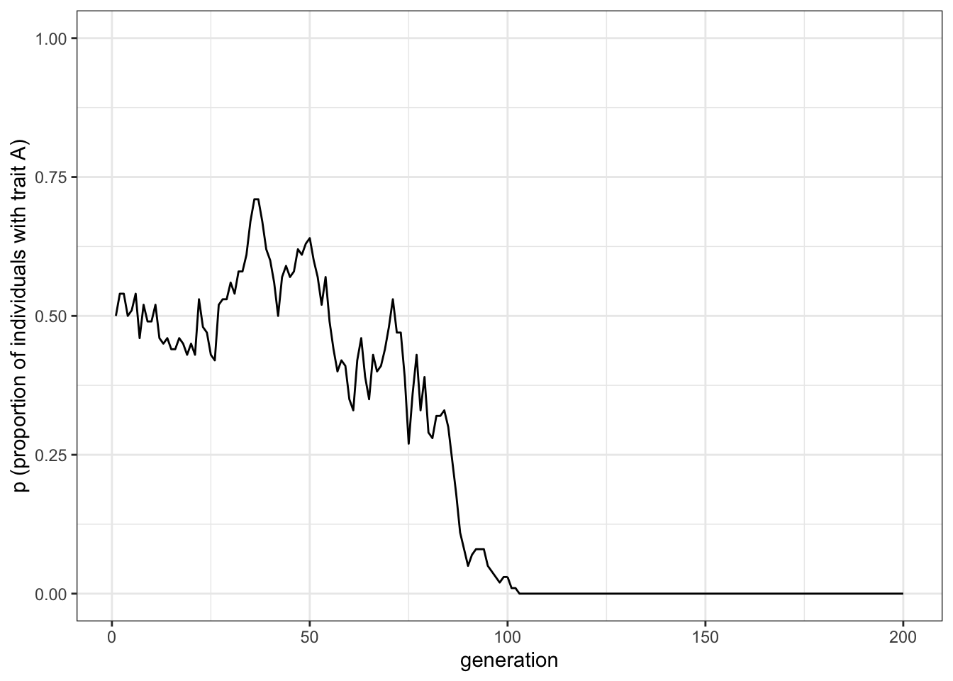
Figure 1.2: Random fluctuations of the proportion of trait A under unbiased cultural transmission
As expected, the plot is different from the simulation we ran before, even though the code is exactly the same. This is due to the stochastic nature of the simulation.
Now let us change the parameters. We can call the simulation and the plotting functions together. The code below reruns and plots the simulation with a much larger \(N\).
data_model <- unbiased_transmission_1(N = 10000, t_max = 200)
plot_single_run(data_model)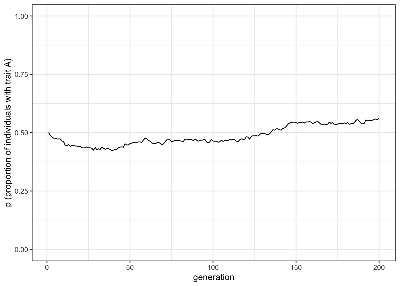
Figure 1.3: Random fluctuations of the proportion of trait A under unbiased cultural transmission and a large population size
As you can see there are much weaker fluctuations. Rarely in a population of \(N = 10000\) will either trait go to fixation. Try re-running the previous code chunk to explore the effect of \(N\) on long-term dynamics.
1.5 Run several independent simulations and plot their results
Wrapping a simulation in a function is good practice because we can easily re-run it with just a single command. From this point on, we can add many more additional computational steps. Say we wanted to re-run the simulation 10 times with the same parameter values to see how many times \(A\) goes to fixation, and how many times \(B\) goes to fixation. Currently, we would have to manually run theunbiased_transmission_1() function 10 times and record somewhere else what happened in each run. Instead, let us automate this just as we have done above.
Let us use a new parameter \(r_{\text{max}}\) to specify the number of independent runs, and use another for-loop to cycle over the \(r_{\text{max}}\) runs. Let’s rewrite the unbiased_transmission_1() function to handle multiple runs. We will call the new function unbiased_transmission_2().
unbiased_transmission_2 <- function(N, t_max, r_max) {
  output <- tibble(generation = rep(1:t_max, r_max),
                   p = as.numeric(rep(NA, t_max * r_max)),
                   run = as.factor(rep(1:r_max, each = t_max)))
  # For each run
  for (r in 1:r_max) {
    # Create first generation
    population <- tibble(trait = sample(c("A", "B"), N, replace = TRUE))

    # Add first generation's p for run r
    output[output$generation == 1 & output$run == r, ]$p <-
      sum(population$trait == "A") / N

    # For each generation
    for (t in 2:t_max) {
      # Copy individuals to previous_population tibble
      previous_population <- population

      # Randomly copy from previous generation
      population <- tibble(trait = sample(previous_population$trait, N, replace = TRUE))

      # Get p and put it into output slot for this generation t and run r
      output[output$generation == t & output$run == r, ]$p <-
        sum(population$trait == "A") / N
    }
  }
  # Export data from function
  output
}
There are a few changes here. First, we need a different output tibble, because we need to store data for all the runs. For that, we initialise the same generation and p columns as before, but with space for all the runs. generation is now built by repeating the count of each generation \(r_{\text{max}}\) times, and p is NA repeated for all generations, for all runs.
We also need a new column called run that keeps track of which run the data in the other two columns belongs to. Note that the definition of run is preceded by as.factor(). This specifies the type of data to put in the run column. We want run to be a ‘factor’ or categorical variable so that, even if runs are labelled with numbers (1, 2, 3…), this should not be misinterpreted as a continuous, real number: there is no sense in which run 2 is twice as ‘runny’ as run 1, or run 3 half as ‘runny’ as run 6. Runs could equally have been labelled using letters, or any other arbitrary scheme. While omitting as.factor() does not make any difference when running the simulation, it would create problems when plotting the data because ggplot would treat runs as continuous real numbers rather than discrete categories (you can see this yourself by modifying the definition of output in the previous code chunk). This is a good example of why it is important to have a clear understanding of your data before trying to plot or analyse them.
Going back to the function, we then set up a loop that executes once for each run. The code within this loop is mostly the same as before, except that we now use the [output$generation == t & output$run == r, ] notation to put \(p\) into the right place in output.
The plotting function is also changed to handle multiple runs:
plot_multiple_runs <- function(data_model) {
  ggplot(data = data_model, aes(y = p, x = generation)) +
    geom_line(aes(colour = run)) +
    stat_summary(fun = mean, geom = "line", size = 1) +
    ylim(c(0, 1)) +
    theme_bw() +
    labs(y = "p (proportion of individuals with trait A)")
}
To understand how the above code works, we need to explain the general functioning of ggplot. As explained above, aes() specifies the ‘aesthetics,’ or how the data are mapped to different elements in the plot (e.g. which column contains information about the position along the x or y axis). This is independent of the possible visual representations of this mapping, or ‘geoms.’ If we declare specific aesthetics when we call ggplot(), these aesthetics will be applied to all geoms we call afterwards. Alternatively, we can specify the aesthetics in the geom itself. For example this:
ggplot(data = output, aes(y = p, x = generation)) +
  geom_line() +
  geom_point()
is equivalent to this:
ggplot(data = output) +
  geom_line(aes(y = p, x = generation)) +
  geom_point(aes(y = p, x = generation))
We can use this property to make more complex plots. The plot created in plot_multiple_runs() has two geoms. The first geom is geom_line(). This inherits the aesthetics specified in the initial call to ggplot() but also has a new mapping specific to geom_line(), colour = run. This tells ggplot to plot each run line with a different colour. The next command, stat_summary(), calculates the mean of all runs. However, this only inherits the mapping specified in the initial ggplot() call. If in the aesthetic of stat_summary() we had also specified colour = run, it would separate the data by run, and it would calculate the mean of each run. This, though, is just the lines we have already plotted with the geom_line() command. For this reason, we did not put colour = run in the ggplot() call, only in geom_line(). As always, there are various ways to obtain the same result. This code:
ggplot(data = output) +
  geom_line(aes(y = p, x = generation, colour = run)) +
  stat_summary(aes(y = p, x = generation), fun = mean, geom = "line", size = 1)
is equivalent to the code we wrapped in the function above. However, the original code is clearer, as it distinguishes the global mapping, and the mappings specific to each visual representation.
stat_summary() is a generic ggplot function that can be used to plot different statistics to summarise our data. In this case, we want to calculate the mean of the data mapped in \(y\), we want to plot them with a line, and we want this line to be thicker than the lines for the single runs. The default line size for geom_line is 0.5, so size = 1 doubles the thickness.
Let’s now run the function and plot the results for five runs with the same parameters we used at the beginning (\(N=100\) and \(t_{\text{max}}=200\)):
data_model <- unbiased_transmission_2(N = 100, t_max = 200, r_max = 5)
plot_multiple_runs(data_model)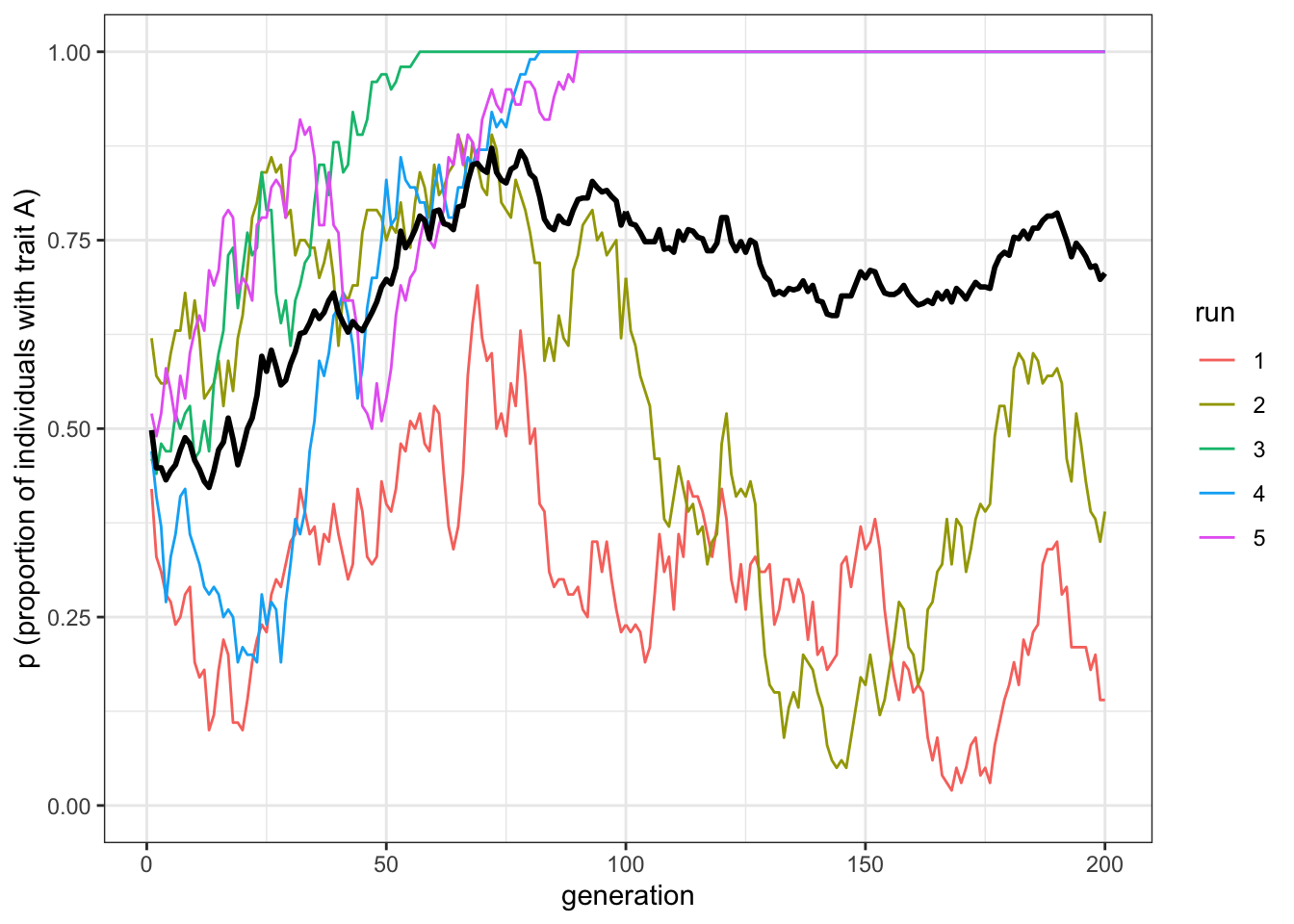
Figure 1.4: Unbiased cultural transmission generates different dynamics in multiple runs
The plot shows five independent runs of our simulation as regular thin lines, along with a thicker black line showing the mean of these lines. Some runs have probably gone to 0 or 1, and the mean should be somewhere in between. The data is stored in data_model, which we can inspect by writing its name.
data_model## # A tibble: 1,000 x 3
## generation p run
## <int> <dbl> <fct>
## 1 1 0.42 1
## 2 2 0.33 1
## 3 3 0.31 1
## 4 4 0.28 1
## 5 5 0.27 1
## 6 6 0.24 1
## 7 7 0.25 1
## 8 8 0.28 1
## 9 9 0.290 1
## 10 10 0.19 1
## # … with 990 more rowsNow let’s run the unbiased_transmission_2() model with \(N = 10000\), to compare with \(N = 100\).
data_model <- unbiased_transmission_2(N = 10000, t_max = 200, r_max = 5)
plot_multiple_runs(data_model)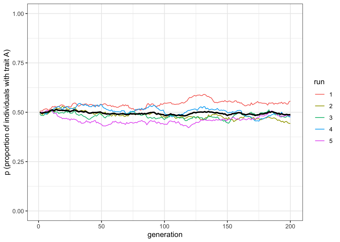
Figure 1.5: Unbiased cultural transmission generates similar dynamics in multiple runs when population sizes are very large
The mean line should be almost exactly at \(p=0.5\) now, with the five independent runs fairly close to it.
1.6 Varying initial conditions
Let’s add one final modification. So far, the starting frequencies of \(A\) and \(B\) have been the same, roughly 0.5 each. But what if we were to start at different initial frequencies of \(A\) and \(B\)? Say, \(p=0.2\) or \(p=0.9\)? Would unbiased transmission keep \(p\) at these initial values, or would it go to \(p=0.5\) as we have found so far?
To find out, we can add another parameter, p_0, which specifies the initial probability of an individual having an \(A\) rather than a \(B\) in the first generation. Previously this was always p_0 = 0.5, but in the new function below we add it to the sample() function to weight the initial allocation of traits.
unbiased_transmission_3 <- function(N, p_0, t_max, r_max) {
  output <- tibble(generation = rep(1:t_max, r_max),
                   p = as.numeric(rep(NA, t_max * r_max)),
                   run = as.factor(rep(1:r_max, each = t_max)))
  # For each run
  for (r in 1:r_max) {
    # Create first generation
    population <- tibble(trait = sample(c("A", "B"), N, replace = TRUE,
                                        prob = c(p_0, 1 - p_0)))

    # Add first generation's p for run r
    output[output$generation == 1 & output$run == r, ]$p <-
      sum(population$trait == "A") / N
    for (t in 2:t_max) {
      # Copy individuals to previous_population tibble
      previous_population <- population

      # Randomly copy from previous generation
      population <- tibble(trait = sample(previous_population$trait, N, replace = TRUE))

      # Get p and put it into output slot for this generation t and run r
      output[output$generation == t & output$run == r, ]$p <-
        sum(population$trait == "A") / N
    }
  }
  # Export data from function
  output
}
unbiased_transmission_3() is almost identical to the previous function. The only changes are the addition of \(p_0\) as an argument to the function, and the \(prob\) argument in the sample() command, which defines the probability of picking each option, in our case \(A\) and \(B\), in the first generation. The probability of \(A\) is now \(p_0\), and the probability of \(B\) is now \(1-p_0\). We can use the same plotting function as before to visualise the result. Let’s see what happens with a different value of \(p_0\), for example \(p_0=0.2\).
data_model <- unbiased_transmission_3(N = 10000, p_0 = 0.2, t_max = 200, r_max = 5)
plot_multiple_runs(data_model)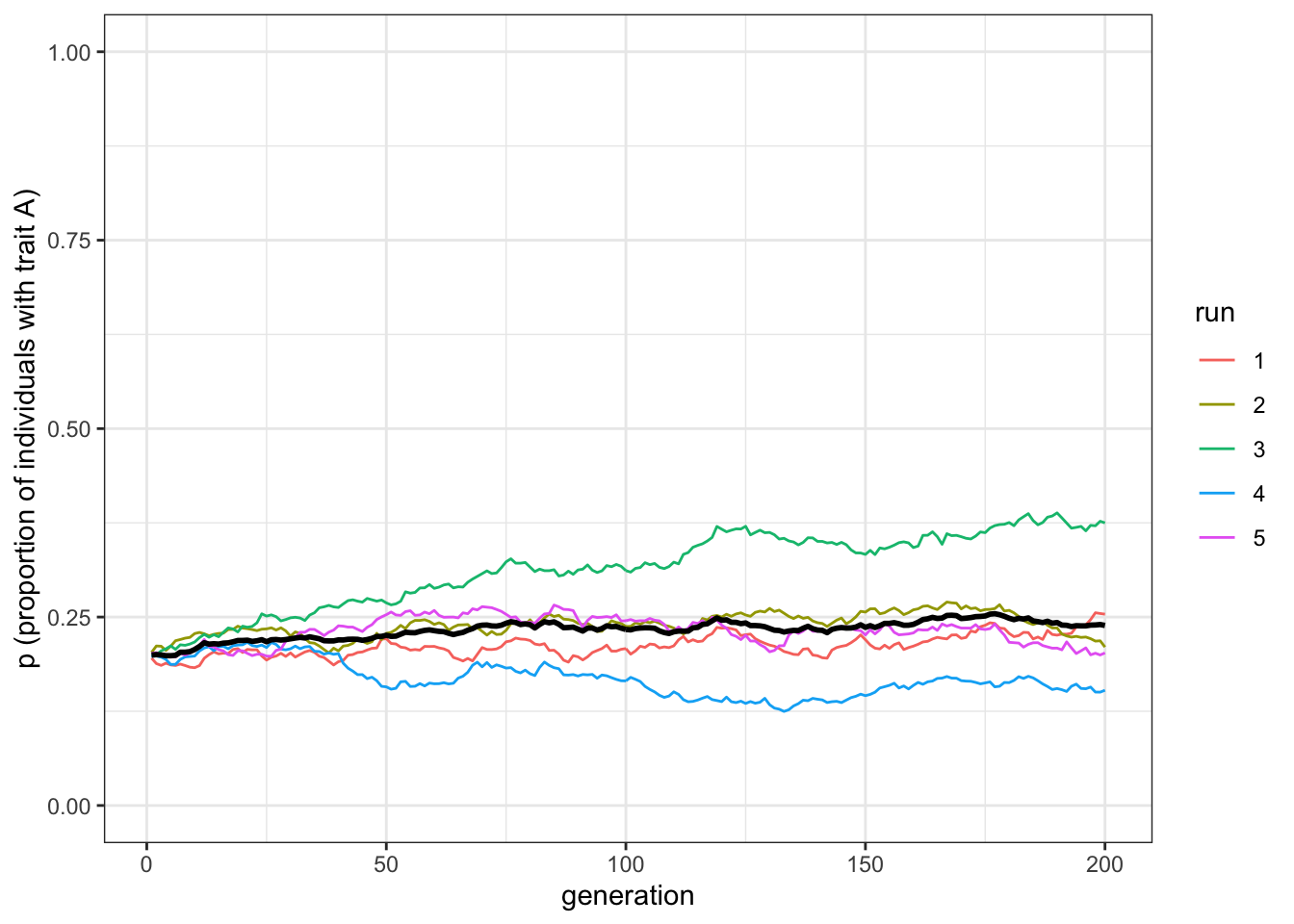
Figure 1.6: Unbiased transmission does not change trait frequencies from the starting conditions, barring random fluctuations
With \(p_0=0.2\), trait frequencies stay at \(p=0.2\). Unbiased transmission is truly non-directional: it maintains trait frequencies at whatever they were in the previous generation, barring random fluctuations caused by small population sizes.
1.7 Summary of the model
Even this extremely simple model provides some valuable insights. First, unbiased transmission does not in itself change trait frequencies. As long as populations are large, trait frequencies remain fairly the same.
Second, the smaller the population size, the more likely traits are to be lost by chance. This is a basic insight from population genetics, known there as genetic drift, but it can also be applied to cultural evolution. Many studies have tested (and some supported) the idea that population size and other demographic factors can shape cultural diversity.
Furthermore, generating expectations about cultural change under simple assumptions like random cultural drift can be useful for detecting non-random patterns like selection. If we don’t have a baseline, we won’t know selection or other directional processes when we see them.
We have also introduced several programming techniques that will be useful in later simulations. We have seen how to use tibbles to hold characteristics of individuals and the outputs of simulations, how to use loops to cycle through generations and simulation runs, how to use sample() to pick randomly from sets of elements, how to wrap simulations in functions to easily re-run them with different parameter values, and how to use ggplot() to plot the results of simulations.
1.8 Further reading
Cavalli-Sforza and Feldman (1981) explored how cultural drift affects cultural evolution, which was extended by Neiman (1995) in an archaeological context. Bentley, Hahn, and Shennan (2004) present models of unbiased transmission for several cultural datasets. Lansing and Cox (2011) and commentaries explore the underlying assumptions of applying random drift to cultural evolution.