Chapter 6 Vertical and horizontal transmission

An important distinction in cultural evolution concerns the pathway of cultural transmission. Vertical cultural transmission occurs when individuals learn from their parents. Oblique cultural transmission occurs when individuals learn from other (non-parental) members of the older generation, such as teachers. Horizontal cultural transmission occurs when individuals learn from members of the same generation.

These terms (vertical, oblique and horizontal) are borrowed from epidemiology, where they are used to describe the transmission of diseases. Cultural traits, like diseases, are interesting in that they have multiple pathways of transmission. While genes spread purely vertically (at least in species like ours; horizontal gene transfer is common in plants and bacteria), cultural traits can spread obliquely and horizontally. These latter pathways can increase the rate at which cultural traits can spread, compared to vertical transmission alone.

In this chapter we will simulate and test this claim, focusing in particular on horizontal cultural transmission: when and why does horizontal transmission increase the rate of spread of a cultural trait compared to vertical cultural transmission?

6.1 Vertical cultural transmission

To simulate vertical cultural transmission we need to decide how people learn from their parents, assuming those two parents possess different combinations of cultural traits. As in previous models, we assume two discrete traits, \(A\) and \(B\). There are then four combinations of traits amongst two parents: both parents have \(A\), both parents have \(B\), mother has \(A\) and father has \(B\), and mother has \(B\) and father has \(A\).

For simplicity, we can assume that when both parents have the same trait, the child adopts that trait. When parents differ, the child faces a choice. To make things more interesting, let’s assume a bias for one trait over the other in such situations (otherwise we would be back to unbiased transmission, and no trait would reliably spread - remember we are interested in how quickly traits spread under vertical vs horizontal transmission).

Hence we assume a probability \(b\) that, when parents differ in their traits such that there is some uncertainty, the child adopts \(A\). With probability \(1-b\) they adopt trait \(B\). When \(b=0.5\), transmission is unbiased. When \(b>0.5\), \(A\) should be favoured; when \(b<0.5\), \(B\) should be favoured. Let’s simulate this and test these predictions.

The following function vertical_transmission() is very similar to previous simulation functions. The explanation follows.

library(tidyverse)

vertical_transmission <- function(N, p_0, b, t_max, r_max) {
  output <- tibble(generation = rep(1:t_max, r_max), 
                   p = as.numeric(rep(NA, t_max * r_max)), 
                   run = as.factor(rep(1:r_max, each = t_max)))
  
  for (r in 1:r_max) {
    # Create first generation
    population <- tibble(trait = sample(c("A", "B"), N, 
                                        replace = TRUE, prob = c(p_0, 1 - p_0)))
    
    # Add first generation's p for run r
    output[output$generation == 1 & output$run == r, ]$p <- 
      sum(population$trait == "A") / N 
    
    for (t in 2:t_max) {
       # Copy individuals to previous_population tibble
      previous_population <- population
      
      # Randomly pick mothers and fathers
      mother <- tibble(trait = sample(previous_population$trait, N, replace = TRUE))  
      father <- tibble(trait = sample(previous_population$trait, N, replace = TRUE)) 
      
      # Prepare next generation
      population <- tibble(trait = as.character(rep(NA, N))) 
      
      # Both parents are A, thus child adopts A
      both_A <- mother$trait == "A" & father$trait == "A"
      if (sum(both_A) > 0) {
        population[both_A, ]$trait <- "A"  
      }
      
      # Both parents are B, thus child adopts B
      both_B <- mother$trait == "B" & father$trait == "B"
      if (sum(both_B) > 0) {
        population[both_B, ]$trait <- "B" 
      }
      # If any empty NA slots (i.e. one A and one B parent) are present
      if (anyNA(population)) {  
        # They adopt A with probability b
        population[is.na(population)[,1],]$trait <- 
          sample(c("A", "B"), sum(is.na(population)), prob = c(b, 1 - b), replace = TRUE)
      }
      
      # Get p and put it into output slot for this generation t and run r
      output[output$generation == t & output$run == r, ]$p <- 
        sum(population$trait == "A") / N 
    }
  }
  # Export data from function
  output 
}

First we set up an output tibble to store the frequency of \(A\) (\(p\)) over \(t_{\text{max}}\) generations and across \(r_{\text{max}}\) runs. As before we create a population tibble to store our \(N\) traits, one per individual.

This time, however, in each generation we create two new tibbles, mother and father. These store the traits of two randomly chosen individuals from the previous_population, one pair for each new individual (notice each individual can be interchangeably either mother or father). We are also assuming random mating here: parents pair up entirely at random. Alternative mating rules are possible, such as assortative cultural mating, where parents preferentially assort based on their cultural trait. We will leave it to readers to create models of this.

Once the mother and father tibbles are created, we can fill in the new individuals’ traits in population. both_A is used to mark with TRUE whether both mother and father have trait \(A\), and (assuming some such cases exist), sets all individuals in population for whom this is true to have trait \(A\). both_B works equivalently for parents who both possess trait \(B\).

The remaining cases (identified as still being NA in the population tibble, with the function anyNA()) must have one \(A\) and one \(B\) parent. We are not concerned with which parent has which in this simple model, so in each of these cases we set the individual’s trait to be \(A\) with probability \(b\) and \(B\) with probability \(1-b\). Again, we leave it to readers to modify the code to have separate probabilities for maternal and paternal transmission.

Once all generations are finished, we export the output tibble as our data. We can use our existing function plot_multiple_runs() from previous chapters to plot the results.

And now run both functions to see what happens. Remember we are interested in how fast the favoured trait spreads, so let’s start it off at a low frequency (\(p_0=0.01\)) so we can see it spreading from rarity. We use a small transmission bias \(b=0.6\) favouring \(A\).

data_model <- vertical_transmission(N = 10000, p_0 = 0.01, b = 0.6, 
                                    t_max = 50, r_max = 5)
plot_multiple_runs(data_model)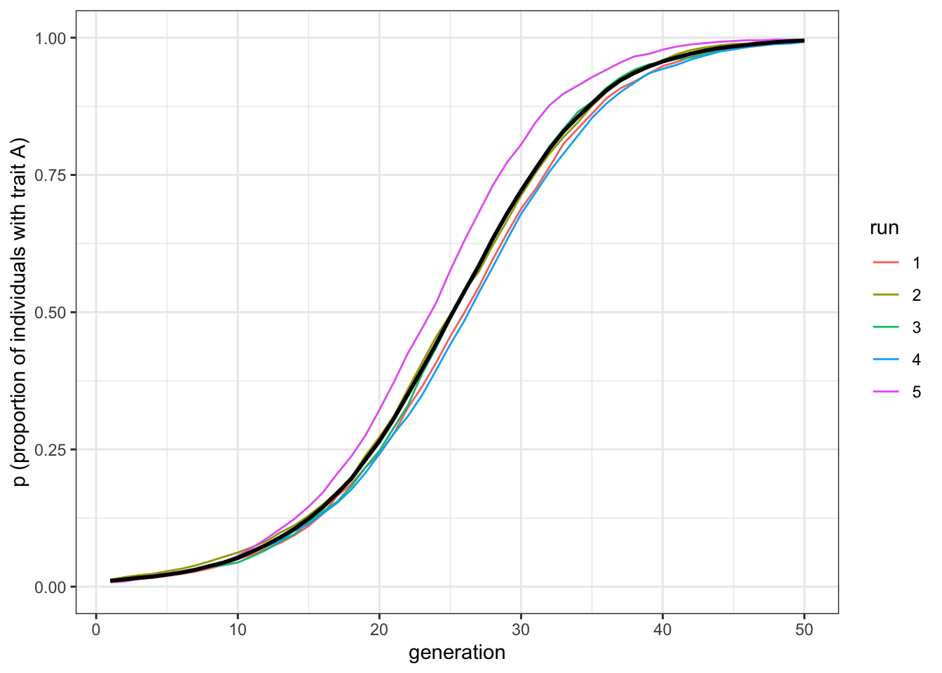

Figure 6.1: The favourite trait, A, spreads in the population under vertical transmission.

Here we can see a gradual spread of the favoured trait \(A\) from \(p=0.01\) to \(p=1\). As in our directly biased transmission model, the diffusion curve is s-shaped. To obtain the same result with two different models is encouraging! We can also test our prediction that when \(b=0.5\), we recreate our unbiased transmission model from Chapter 1:

data_model <- vertical_transmission(N = 10000, p_0 = 0.1, b = 0.5, 
                                    t_max = 50, r_max = 5)
plot_multiple_runs(data_model)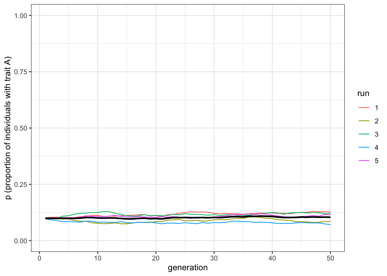

Figure 6.2: When no trait is favoured, there is no change in the frequency of trait A under vertical transmission.

As predicted, there is no change in starting trait frequencies when \(b=0.5\). If you reduce the sample size, you will see much more fluctuation across the runs, with some runs losing \(A\) altogether.

6.2 Horizontal cultural transmission

Now let’s add horizontal cultural transmission to our model. We will add it to vertical cultural transmission, rather than replace vertical with horizontal, so we can compare both in the same model.

First there is vertical transmission as above, with random mating and the parental bias \(b\), to create a new generation. Then, the new generation learns from each other. The key difference between vertical and horizontal transmission is that horizontal cultural transmission can occur from more than two individuals. Let’s assume individuals pick \(n\) other individuals from their generation. We also assume a bias in favour of \(A\) during horizontal transmission. If the learner is \(B\), then for each of the \(n\) demonstrators who have \(A\), there is an independent probability \(g\) that the learner switches to \(A\). If the learner is already \(A\), or if the demonstrator is \(B\), then nothing happens.

The following code implements this horizontal transmission in a new function vertical_horizontal_transmission().

vertical_horizontal_transmission <- function(N, p_0, b, n, g, t_max, r_max) {
  output <- tibble(generation = rep(1:t_max, r_max), 
                   p = as.numeric(rep(NA, t_max * r_max)), 
                   run = as.factor(rep(1:r_max, each = t_max)))
  
  for (r in 1:r_max) {
    # Create first generation
    population <- tibble(trait = sample(c("A", "B"), N, 
                                        replace = TRUE, prob = c(p_0, 1 - p_0)))
    
    # Add first generation's p for run r
    output[output$generation == 1 & output$run == r, ]$p <- 
      sum(population$trait == "A") / N 
    
    for (t in 2:t_max) {
      # Vertical transmission --------------------------------------------------
      
      # Copy individuals to previous_population tibble
      previous_population <- population 
      
      # Randomly pick mothers and fathers
      mother <- tibble(trait = sample(previous_population$trait, N, replace = TRUE))  
      father <- tibble(trait = sample(previous_population$trait, N, replace = TRUE))  
      
      # Prepare next generation
      population <- tibble(trait = as.character(rep(NA, N))) 
      
      # Both parents are A, thus child adopts A
      both_A <- mother$trait == "A" & father$trait == "A"
      if (sum(both_A) > 0) {
        population[both_A, ]$trait <- "A"  
      }
      
      # Both parents are B, thus child adopts B
      both_B <- mother$trait == "B" & father$trait == "B"
      if (sum(both_B) > 0) {
        population[both_B, ]$trait <- "B" 
      }
      # If any empty NA slots (i.e. one A and one B parent) are present
      if (anyNA(population)) {  
        # They adopt A with probability b
        population[is.na(population)[,1],]$trait <- 
          sample(c("A", "B"), sum(is.na(population)), prob = c(b, 1 - b), replace = TRUE)
      }
      
      # Horizontal transmission ------------------------------------------------
      
      # Previous_population are children before horizontal transmission
      previous_population <- population 
      
      # N_B = number of Bs
      N_B <- length(previous_population$trait[previous_population$trait == "B"])  
      
      # If there are B individuals to switch, and n is not zero
      if (N_B > 0 & n > 0) {  
        # For each B individual...
        for (i in 1:N_B) {  
          # Pick n demonstrators
          demonstrator <- sample(previous_population$trait, n, replace = TRUE)
          # Get probability g
          copy <- sample(c(TRUE, FALSE), n, prob = c(g, 1-g), replace = TRUE) 
          # if any demonstrators with A are to be copied
          if ( sum(demonstrator == "A" & copy == TRUE) > 0 ) {  
            # The B individual switches to A
            population[previous_population$trait == "B",]$trait[i] <- "A"  
          }
        
        }
      }
      # Get p and put it into output slot for this generation t and run r
      output[output$generation == t & output$run == r, ]$p <- 
        sum(population$trait == "A") / N 
    }
  }
  # Export data from function
  output 
}

The first part of this code is identical to vertical_transmission(). Then there is horizontal transmission. We put population into previous_population again, but now population contains the individuals after horizontal transmission, and previous_population contains the individuals before. N_B holds the individuals in previous_population who are \(B\), as they are the only ones we need to concern ourselves with (\(A\) individuals do not change). If there are such individuals (\(N_B>0\)), and individuals are learning from at least one individual (\(n>0\)), then for each individual we pick \(n\) demonstrators, and if any of those demonstrators are \(A\) plus probability \(g\) is fulfilled, we set the individual to \(A\).

Running horizontal transmission with \(n=5\) and \(g=0.1\) and without vertical transmission bias (\(b=0.5\)) causes, as expected, \(A\) to spread.

data_model <- vertical_horizontal_transmission(N = 5000, p_0 = 0.01, b = 0.5, n = 5, 
                                               g = 0.1, t_max = 50, r_max = 5)
plot_multiple_runs(data_model)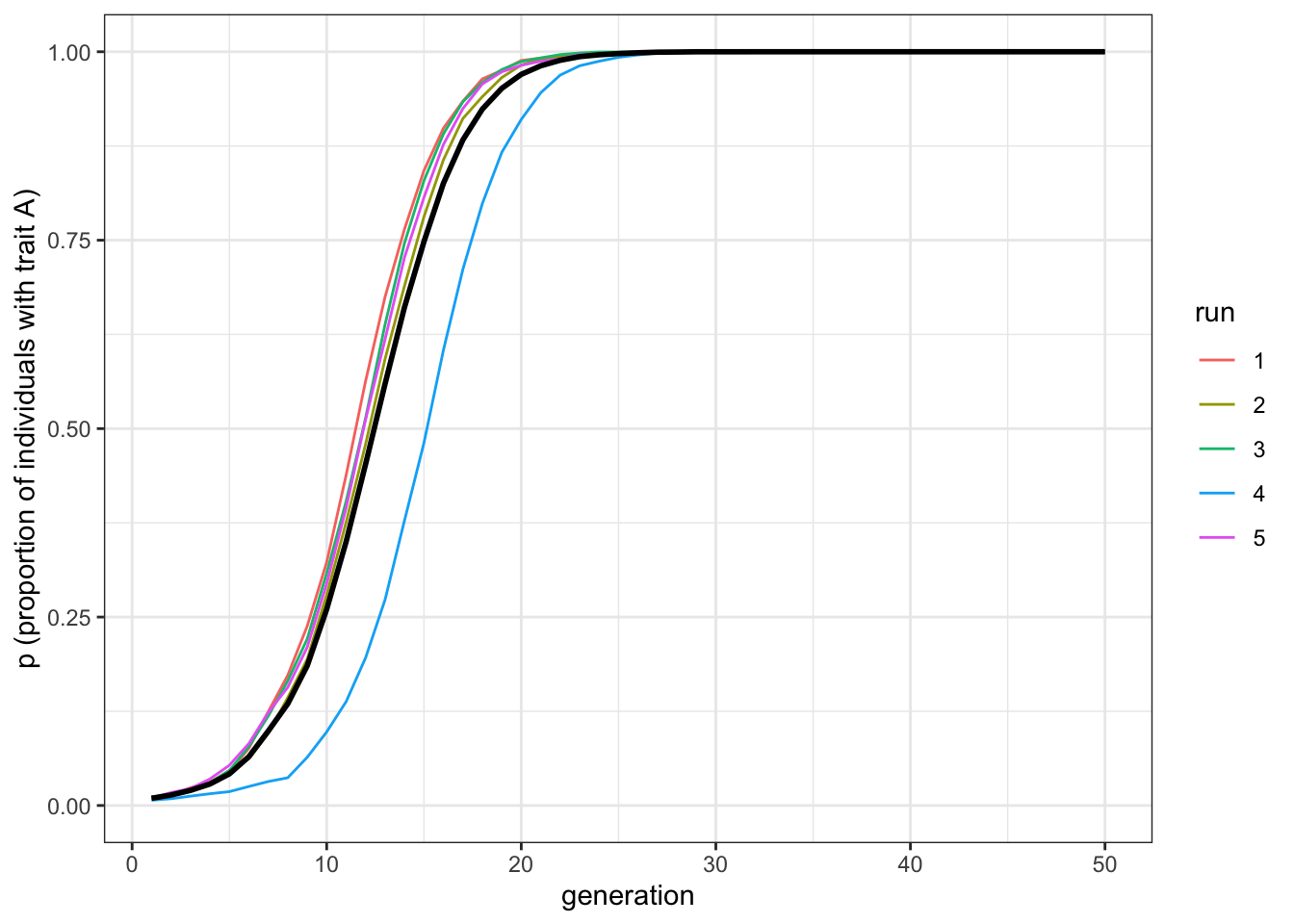

Figure 6.3: The favourite trait, A, spreads in the population under horizontal transmission.

This plot above confirms that horizontal cultural transmission, with some direct bias in the form of \(g\), again generates an s-shaped curve and causes the favoured trait to spread. But we haven’t yet done what we set out to do, which is compare the speed of the different pathways. The following code generates three datasets, one with only vertical transmission and \(b=0.6\), one with only horizontal transmission with \(n=2\) and \(g=0.1\) which is roughly equivalent to two parents and a bias of \(b=0.6\) (0.1 higher than unbiased), and one with only horizontal transmission with \(n=5\) and \(g=0.1\).

data_model_v <- vertical_horizontal_transmission(N = 5000, p_0 = 0.01, b = 0.6, n = 0, 
                                                 g = 0, t_max = 50, r_max = 5)

data_model_hn2 <- vertical_horizontal_transmission(N = 5000, p_0 = 0.01, b = 0.5, n = 2, 
                                                   g = 0.1, t_max = 50, r_max = 5)

data_model_hn5 <- vertical_horizontal_transmission(N = 5000, p_0 = 0.01, b = 0.5, n = 5, 
                                                   g = 0.1, t_max = 50, r_max = 5)

plot_multiple_runs(data_model_v)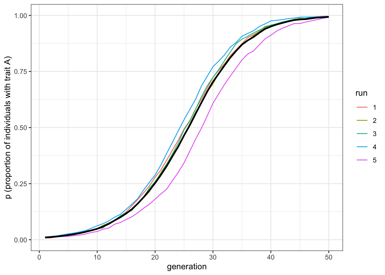

Figure 6.4: The favourite trait, A, spreads in the population under vertical transmission only.

plot_multiple_runs(data_model_hn2)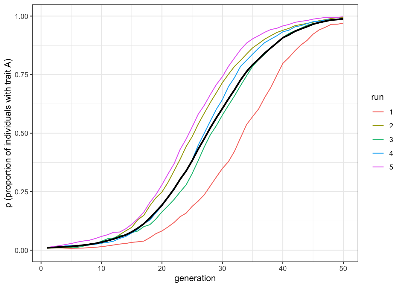

Figure 6.5: Given an equivalent bias strength and two demonstrators, the favourite trait, A, spreads under horizontal transmission at the same speed than in the vertical transmission scenario.

plot_multiple_runs(data_model_hn5)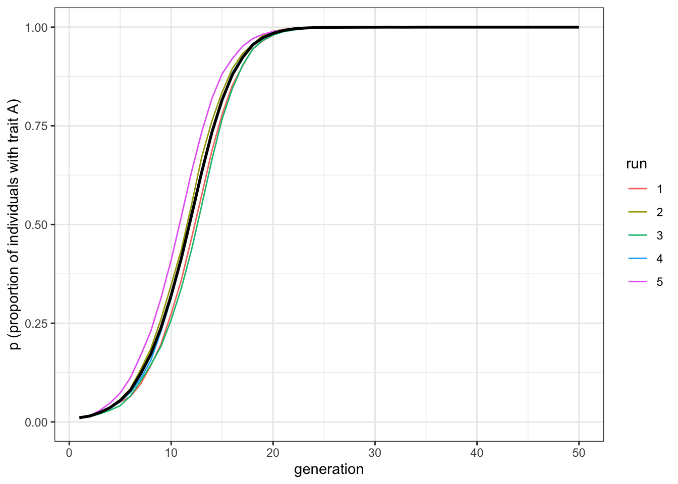

Figure 6.6: Given an equivalent bias strength and five demonstrators, the favourite trait, A, spreads under horizontal transmission faster than in the vertical transmission scenario.

The first two plots should be very similar. Horizontal cultural transmission from \(n=2\) demonstrators is equivalent to vertical cultural transmission, which of course also features two demonstrators, when both pathways have similarly strong direct biases. The third plot shows that increasing the number of demonstrators makes favoured traits spread more rapidly under horizontal transmission, without changing the strength of the biases. Of course, changing the relative strength of the vertical and horizontal biases (\(b\) and \(g\) respectively) also affects the relative speed. But all else being equal, horizontal transmission with \(n>2\) is faster than vertical transmission.

6.3 Summary of the model

This model has combined directly biased transmission with vertical and horizontal transmission pathways. The vertical transmission model recreates the patterns from our previous unbiased and directly biased transmission, but explicitly modelling parents and their offspring. Although there were no differences, our vertical transmission model could be modified easily to study different kinds of parental bias (e.g. making maternal influence stronger than paternal influence), or different types of non-random mating.

Our horizontal transmission model is similar to the conformist bias simulated in Chapter 4, but slightly different - there is no disproportionate majority copying, and instead one trait is favoured when learning from \(n\) demonstrators. Comparing the two pathways, we can see that horizontal cultural transmission is faster than vertical cultural transmission largely because it allows individuals to learn from more than two demonstrators.

6.4 Further reading

The above models are based on those by Cavalli-Sforza and Feldman (1981). Their vertical cultural transmission models feature bias parameters for each combination of matings (\(b_0\), \(b_1\), \(b_2\) and \(b_3\)); our \(b\) is their \(b_1\) and \(b_2\). Their horizontal transmission model also features \(n\) and \(g\), which have the same definitions as here. Subsequent models in that volume examine assortative cultural mating and oblique transmission, although the latter is similar to horizontal transmission.